14-4 Incrementing the Coordinates on the Hilbert Curve

Given the (x, y) coordinates of a point on the order n Hilbert curve, how can one find the coordinates of the next point? One way is to convert (x, y) to s, add 1 to s, and then convert the new value of s back to (x, y), using algorithms given above.

A slightly (but not dramatically) better way is based on the fact that as one moves along the Hilbert curve, at each step either x or y, but not both, is either incremented or decremented (by 1). The algorithm to be described scans the coordinate numbers from left to right to determine the type of U-curve that the rightmost two bits are on. Then, based on the U-curve and the value of the rightmost two bits, it increments or decrements either x or y.

That's basically it, but there is a complication when the path is at the end of a U-curve (which happens once every four steps). At this point, the direction to take is determined by the previous bits of x and y and by the higher order U-curve with which these bits are associated. If that point is also at the end of its U-curve, then the previous bits and the U-curve there determine the direction to take, and so on.

Table 14-7 describes this algorithm. In this table, the A, B, C, and D denote the U-curves as shown in Table 14-1 on page 246. To use the table, first pad x and y with leading zeros so they are n bits long, where n is the order of the Hilbert curve. Start in state A and scan the bits of x and y from left to right. The first row of Table 14-7 means that if the current state is A and the currently scanned bits are (0, 0), then set a variable to indicate to increment y, and enter state B. The other rows are interpreted similarly, with a suffix minus sign indicating to decrement the associated coordinate. A dash in the third column means do not alter the variable that keeps track of the coordinate changes.

After scanning the last (rightmost) bits of x and y, increment or decrement the appropriate coordinate as indicated by the final value of the variable.

A C program implementing these steps is shown in Figure 14-11. Variable dx is initialized in such a way that if invoked many times, the algorithm cycles around, generating the same Hilbert curve over and over again. (However, the step that connects one cycle to the next is not a unit step.)

Figure 14-11 Program for taking one step on the Hilbert curve.

void hil_inc_xy(unsigned *xp, unsigned *yp, int n) {

   int i;

   unsigned x, y, state, dx, dy, row, dochange;

   x = *xp;

   y = *yp;

   state = 0;                   // Initialize.

   dx = -((1 << n) - 1);      ?// Init. -(2**n - 1).

   dy = 0;

   for (i = n-1; i >= 0; i--) {         // Do n times.

      row = 4*state | 2*((x >> i) & 1) | (y >> i) & 1;

      dochange = (0xBDDB >> row) & 1;

      if (dochange) {

         dx = ((0x16451659 >> 2*row) & 3) - 1;

         dy = ((0x51166516 >> 2*row) & 3) - 1;

      state = (0x8FE65831 >> 2*row) & 3;

  ?xp = *xp + dx;

  ?yp = *yp + dy;

Table 14-7. Taking one step on the Hilbert curve
If the current state is	and the next (to right) two bits of (x, y) are	then prepare to inc/dec	and enter state
A	(0, 0)	y+	B
A	(0, 1)	x+	A
A	(1, 0)	?/p>	D
A	(1, 1)	y-	A
B	(0, 0)	x+	A
B	(0, 1)	?/p>	C
B	(1, 0)	y+	B
B	(1, 1)	x-	B
C	(0, 0)	y+	C
C	(0, 1)	?/p>	B
C	(1, 0)	x-	C
C	(1, 1)	y-	D
D	(0, 0)	x+	D
D	(0, 1)	y-	D
D	(1, 0)	?/p>	A
D	(1, 1)	x-	C

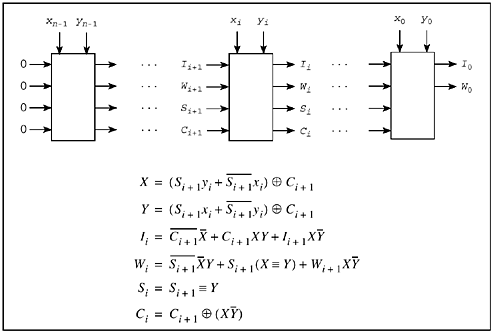
Table 14-7 can readily be implemented in logic, as shown in Figure 14-12. In this figure, the variables have the following meanings:

Figure 14-12. Logic circuit for incrementing (x, y) by one step along the Hilbert curve.

graphics/14fig12.gif

x_i:	Bit i of input x.
y_i:	Bit i of input y.
X, Y:	x_i and y_i swapped and complemented, according to S_i₊₁ and C_i₊₁.
I:	If 1, increment; if 0, decrement (by 1).
W:	If 1, increment or decrement x; if 0, increment or decrement y.
S:	If 1, swap x_i and y_i.
C:	If 1, complement x_i and y_i.

S and C together identify the "state" of Table 14-7, with (C, S) = (0, 0), (0, 1), (1, 0), and (1, 1) denoting states A, B, C, and D, respectively. The output signals are I₀ and W₀, which tell, respectively, whether to increment or decrement, and which variable to change. (In addition to the logic shown, an incrementer/decrementer circuit is required, with MUX's to route either x or y to the incrementer/ decrementer, and a circuit to route the altered value back to the register that holds x or y. Alternatively, two incrementer/decrementer circuits could be used.)