The pedigree chart shows someone's ancestors, in this case those of Dusty, whose two parents are Honey Bear and Brandy. Brandy's parents are Nuggett and Coyote, who are Dusty's grandparents on her father's side. The chart continues one more generation farther back to the great-grandparents. By the nature of things, we know that the pedigree chart is normally two-way branching, though this does not allow for inbreeding. When that occurs we no longer have a tree structure unless we insist that each occurrence of breeding is separately listed. Inbreeding may occur frequently when describing family histories of flowers or animals.
The lineal chart of figure 5.1(b), though it has nothing to do with people, is still a genealogy. It describes, in somewhat abbreviated form, the ancestry of the modern European languages. Thus, this is a chart of descendants rather than ancestors and each item can produce several others. Latin, for instance, is the forebear of Spanish, French, Italian and Rumanian. Proto Indo-European is a prehistoric language presumed to have existed in the fifth millenium B.C. This tree does not have the regular structure of the pedigree chart, but it is a tree structure nevertheless .
With these two examples as motivation let us define formally what we mean by a tree.
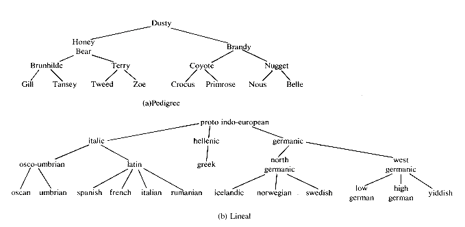
Figure 5.1 Two Types of Geneological Charts
Definition: A tree is a finite set of one or more nodes such that: (i) there is a specially designated node called the root; (ii) the remaining nodes are partitioned into n  0 disjoint sets T1, ...,Tn where each of these sets is a tree. T1, ...,Tn are called the subtrees of the root.
Again we have an instance of a recursive definition (compare this with the definition of a generalized list in section 4.9). If we return to Figure 5.1 we see that the roots of the trees are Dusty and Proto Indo-European. Tree (a) has two subtrees whose roots are Honey Bear and Brandy while tree (b) has 3 subtrees with roots Italic, Hellenic, and Germanic. The condition that T1, ...,Tn be disjoint sets prohibits subtrees from ever connecting together (no cross breeding). It follows that every item in a tree is the root of some subtree of the whole. For instance, West Germanic is the root of a subtree of Germanic which itself has three subtrees with roots: Low German, High German and Yiddish. Yiddish is a root of a tree with no subtrees.
There are many terms which are often used when referring to trees. A node stands for the item of information plus the branches to other items. Consider the tree in figure 5.2. This tree has 13 nodes, each item of data being a single letter for convenience. The root is A and we will normally draw trees with the root at the top. The number of subtrees of a node is called its degree. The degree of A is 3, of C is 1 and of F is zero. Nodes that have degree zero are called leaf or terminal nodes. {K,L,F,G,M,I,J} is the set of leaf nodes. Alternatively, the other nodes are referred to as nonterminals. The roots of the subtrees of a node, X, are the children of X. X is the parent of its children. Thus, the children of D are H, I, J; the parent of D is A. Children of the same parent are said to be siblings. H, I and J are siblings. We can extend this terminology if we need to so that we can ask for the grandparent of M which is D, etc. The degree of a tree is the maximum degree of the nodes in the tree. The tree of figure 5.2 has degree 3. The ancestors of a node are all the nodes along the path from the root to that node. The ancestors of M are A, D and H.
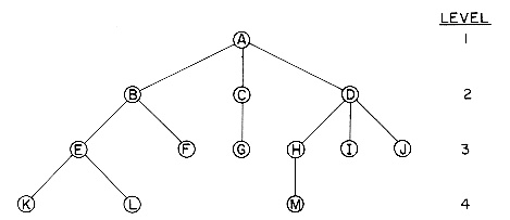
Figure 5.2 A Sample Tree
The level of a node is defined by initially letting the root be at level one. If a node is at level l, then its children are at level l + 1. Figure 5.2 shows the levels of all nodes in that tree. The height or depth of a tree is defined to be the maximum level of any node in the tree.
A forest is a set of n
There are other ways to draw a tree. One useful way is as a list. The tree of figure 5.2 could be written as the list
(A(B(E(K,L),F),C(G),D(H(M),I,J)))
The information in the root node comes first followed by a list of the subtrees of that node.
Now, how do we represent a tree in memory? If we wish to use linked lists, then a node must have a varying number of fields depending upon the number of branches.
However it is often simpler to write algorithms for a data representation where the node size is fixed. Using data and pointer fields we can represent a tree using the fixed node size list structure we devised in Chapter 4. The list representation for the tree of Figure 5.2 is on page 222. We can now make use of many of the general procedures that we originally wrote for handling lists. Thus, the data object tree is a special instance of the data object list and we can specialize the list representation scheme to them. In a later section we will see that another data object which can be used to represent a tree is the data object binary tree.
A binary tree is an important type of tree structure which occurs very often. It is characterized by the fact that any node can have at most two branches, i.e., there is no node with degree greater than two. For binary trees we distinguish between the subtree on the left and on the right, whereas for trees the order of the subtrees was irrelevant. Also a binary tree may have zero nodes. Thus a binary tree is really a different object than a tree.
Definition: A binary tree is a finite set of nodes which is either empty or consists of a root and two disjoint binary trees called the left subtree and the right subtree.
Using the notation introduced in chapter one we can define the data structure binary tree as follows:
This set of axioms defines only a minimal set of operations on binary trees. Other operations can usually be built in terms of these. See exercise 35 for an example.
The distinctions between a binary tree and a tree should be analyzed. First of all there is no tree having zero nodes, but there is an empty binary tree. The two binary trees below
are different. The first one has an empty right subtree while the second has an empty left subtree. If the above are regarded as trees, then they are the same despite the fact that they are drawn slightly differently.
Figure 5.3 shows two sample binary trees. These two trees are special kinds of binary trees. The first is a skewed tree, skewed to the left and there is a corresponding one which skews to the right. Tree 5.3b is called a complete binary tree. This kind of binary tree will be defined formally later on. Notice that all terminal nodes are on adjacent levels. The terms that we introduced for trees such as: degree, level, height, leaf, parent, and child all apply to binary trees in the natural way. Before examining data representations for binary trees, let us first make some relevant observations regarding such trees. First, what is the maximum number of nodes in a binary tree of depth k?
Lemma 5.1
(i) The maximum number of nodes on level i of a binary tree is 2i-1, i
(ii) The maximum number of nodes in a binary tree of depth k is 2k - 1, k
Proof:
(i) The proof is by induction on i.
Induction Base: The root is the only node on level i= 1. Hence the maximum number of nodes on level i = 1 is 2
Induction Hypothesis: For all j, 1
Induction Step: The maximum number of nodes on level i - 1 is 2i - 2, by the induction hypothesis. Since each node in a binary tree has maximum degree 2, the maximum number of nodes on level i is 2 times the maximum number on level i - 1 or 2i-1.
(ii) The maximum number of nodes in a binary tree of depth k is
Next, let us examine the relationship between the number of terminal nodes and the number of nodes of degree 2 in a binary tree.
Lemma 5.2: For any nonempty binary tree, T, if no is the number of ter minal nodes and n2 the number of nodes of degree 2, then n0 = n2 + 1.
Proof: Let n1 be the number of nodes of degree 1 and n the total number of nodes. Since all nodes in T are of degree
n = n0 + n1 + n2
If we count the number of branches in a binary tree, we see that every node except for the root has a branch leading into it. If B is the number of branches, then n = B + 1. All branches emanate either from a node of degree one or from a node of degree 2. Thus, B = n1 + 2n2. Hence, we obtain
n = 1 + n1 + 2n2
Subtracting (5.2) from (5.1) and rearranging terms we get
n0= n2 + 1
In Figure 5.3(a) n0 = 1 and n2 = 0 while in Figure 5.3(b) n0 = 5 and n2 = 4.
As we continue our discussion of binary trees, we shall derive some other interesting properties.
A full binary tree of depth k is a binary tree of depth k having 2k - 1 nodes. By Lemma 5.1, this is the maximum number of nodes such a binary tree can have. Figure 5.4 shows a full binary tree of depth 4. A very elegant sequential representation for such binary trees results rom sequentially numbering the nodes, starting with nodes on level 1, then those on level 2 and so on. Nodes on any level are numbered from left to right (see figure 5.4). This numbering scheme gives us the definition of a complete binary tree. A binary tree with n nodes and of depth k is complete iff its nodes correspond to the nodes which re numbered one to n in the full binary tree of depth k. The nodes may now be stored in a one dimensional array, TREE, with the node umbered i being stored in TREE(i). Lemma 5.3 enables us to easily determine the locations of the parent, left child and right child of any node i in the binary tree.
Lemma 5.3: If a complete binary tree with n nodes (i.e., depth= [log2n] + 1) is represented sequentially as above then for any node with index i, 1
(i) PARENT(i) is at [i/2] if i
(ii) LCHILD(i) is at 2i if 2i
(iii) RCHILD(i) is at 2i + 1 if 2i + 1
Proof: We prove (ii). (iii) is an immediate consequence of (ii) and the numberin g of nodes on the same level from left to right. (i) follows from (ii) and (iii). We prove (ii) by induction on i. For i= 1, clearly the left child is at 2 unless 2 > n in which case 1 has no left child. Now assume that for all j, 1
This representation can clearly be used for all binary trees though in most cases there will be a lot of unutilized space. For complete binary trees the representation is ideal as no space is wasted. For the skewed tree of figure 5.3(a), however, less than half the array is utilized. In the worst case a skewed tree of depth k will require 2k - 1 spaces. Of these only k will be occupied.
While the above representation appears to be good for complete binary trees it is wasteful for many other binary trees. In addition, the representation suffers from the general inadequacies of sequential representations. Insertion or deletion of nodes from the middle of a tree requires the movement of potentially many nodes to reflect the change in level number of these nodes. These problems can be easily overcome through the use of a linked representation. Each node will have three fields LCHILD, DATA and RCHILD as below:
While this node structure will make it difficult to determine the parent of a node, we shall see that for most applications, it is adequate. In case it is necessary to be able to determine the parent of random nodes. then a fourth field PARENT may be included. The representation of the binary trees of figure 5.3 using this node structure is given in figure 5.6.
There are many operations that we often want to perform on trees. One notion that arises frequently is the idea of traversing a tree or visiting each node in the tree exactly once. A full traversal produces a linear order for the information in a tree. This linear order may be familiar and useful. When traversing a binary tree we want to treat each node and its subtrees in the same fashion. If we let L, D, R stand for moving left, printing the data, and moving right when at a node then there are six possible combinations of traversal: LDR, LRD, DLR, DRL, RDL, and RLD. If we adopt the convention that we traverse left before right then only three traversals remain: LDR, LRD and DLR. To these we assign the names inorder, postorder and preorder because there is a natural correspondence between these traversals and producing the infix, postfix and prefix forms of an expression. Consider the binary tree of figure 5.7. This tree contains an arithmetic expression with binary operators: add(+), multiply(*), divide(/), exponentiation(**) and variables A, B, C, D, and E. We will not worry for now how this binary tree was formed, but assume that it is available. We will define three types of traversals and show the results for this tree.
Inorder Traversal: informally this calls for moving down the tree towards the left until you can go no farther. Then you "visit" the node, move one node to the right and continue again. If you cannot move to the right, go back one more node. A precise way of describing this traversal is to write it as a recursive procedure.
Recursion is an elegant device for describing this traversal. Let us trace how INORDER works on the tree of figure 5.7.
The elements get printed in the order
A/B ** C * D + E
which is the infix form of the expression.
A second form of traversal is preorder:
In words we would say "visit a node, traverse left and continue again. When you cannot continue, move right and begin again or move back until you can move right and resume." The nodes of figure 5.7 would be printed in preorder as
+* / A ** B C D E
which we recognize as the prefix form of the expression.
At this point it should be easy to guess the next traversal method which is called postorder:
The output produced by POSTORDER is
A B C ** / D * E +
which is the postfix form of our expression.
Though we have written these three algorithms using recursion, it is very easy to produce an equivalent nonrecursive procedure. Let us take inorder as an example. To simulate the recursion we need a stack which will hold pairs of values (pointer, returnad) where pointer points to a node in the tree and returnad to the place where the algorithm should resume after an end is encountered. We replace every recursive call by a mechanism which places the new pair (pointer, returnad) onto the stack and goes to the beginning; and where there is a return or end we insert code which deletes the top pair from the stack if possible and either ends or branches to returnad (see section 4.10 for the exact details).
Though this procedure seems highly unstructured its virtue is that it is semiautomatically produced from the recursive version using a fixed set of rules. Our faith in the correctness of this program can be justified
if we first prove the correctness of the original version and then prove that the transformation rules result in a correct and equivalent program. Also we can simplify this program after we make some observations about its behavior. For every pair (T1,L3) in the stack when we come to label L3 this pair will be removed. All such consecutive pairs will be removed until either i gets set to zero or we reach a pair (T2,L2). Therefore, the presence of L3 pairs is useful in no way and we can delete that part of the algorithm. This means we can eliminate the two lines of code following print (DATA(T)). We next observe that this leaves us with only one return address, L2, so we need not place that on the stack either. Our new version now looks like:
This program is considerably simpler than the previous version, but it may still offend some people because of the seemingly undisciplined use of go to's. A SPARKS version without this statement would be:
In going from the recursive version to the iterative version INORDER3 one undesirable side effect has crept in. While in the recursive version T was left pointing to the root of the tree, this is not the case when INORDER3 terminates. This may readily be corrected by introducing another variable P which is used in place of T during the traversal.
What are the computing time and storage requirements of INORDER3 ? Let n be the number of nodes in T. If we consider the action of the above algorithm, we note that every node of the tree is placed on the stack once. Thus, the statements STACK(i)
2n0 + n1 = n0 + n1 + n2 + 1 = n + 1.
So every step will be executed no more than some small constant times n or O(n). With some further modifications we can lower the constant (see exercises). The space required for the stack is equal to the depth of T. This is at most n.
Before we leave the topic of tree traversal, we shall consider one final question. Is it possible to traverse binary trees without the use of extra space for a stack? One simple solution is to add a PARENT field to each node. Then we can trace our way back up to any root and down again. Another solution which requires two bits per node is given in section 5.6. If the allocation of this extra space is too costly then we can use the method of algorithm MARK2 of section 4.10. No extra storage is required since during processing the LCHILD and RCHILD fields are used to maintain the paths back to the root. The stack of addresses is stored in the leaf nodes. The exercises examine this algorithm more closely.
Using the definition of a binary tree and the recursive version of the traversals, we can easily write other routines for working with binary trees. For instance, if we want to produce an exact copy of a given binary tree we can modify the postorder traversal algorithm only slightly to get:
Another problem that is especially easy to solve using recursion is determining the equivalence of two binary trees. Binary trees are equivalent if they have the same topology and the information in corresponding nodes is identical. By the same topology we mean that every branch in one tree corresponds to a branch in the second in the same order. Algorithm EQUAL traverses the binary trees in preorder, though any order could be used.
We have seen that binary trees arise naturally with genealogical information and further that there is a natural relationship between the tree traversals and various forms of expressions. There are many other
instances when binary trees are important, and we will look briefly at two of them now. The first problem has to do with processing a list of alphabetic data, say a list of variable names such as
X1, I, J, Z, FST, X2, K.
We will grow a binary tree as we process these names in such a way that for each new name we do the following: compare it to the root and if the new name alphabetically precedes the name at the root then move left or else move right; continue making comparisons until we fall off an end of the tree; then create a new node and attach it to the tree in that position. The sequence of binary trees obtained for the above data is given in figure 5.8. Given the tree in figure 5.8(g) consider the order of the identifiers if they were printed out using an inorder traversal
FST, I, J, K, X1, X2, Z
So by growing the tree in this way we turn inorder into a sorting method. In Chapter 9 we shall prove that this method works in general.
As a second example of the usefulness of binary trees, consider the set of formulas one can construct by taking variables x1,x2,x3, ... and the operators
x1
is a formula (read "x1 or x2 and not X3"). If xl and X3 are false and x2 is true, then the value of this expression is
The satisfiability problem for formulas of the propositional calculus asks if there is an assignment of values to the variables which causes the value of the expression to be true. This problem is of great historical interest in computer science. It was originally used by Newell, Shaw and Simon in the late 1950's to show the viability of heuristic programming (the Logic Theorist).
Again, let us assume that our formula is already in a binary tree, say
(x1
in the tree
The inorder of this tree is x1
To evaluate an expression one method would traverse the tree in postorder, evaluating subtrees until the entire expression is reduced to a single value. This corresponds to the postfix evaluation of an arithmetic expression that we saw in section 3.3. Viewing this from the perspective of the tree representation, for every node we reach, the values of its arguments (or children) have already been computed. So when we reach the v node on level two, the values of x1
For the purposes of this algorithm we assume each node has four fields:
where LCHILD, DATA, RCHILD are as before and VAL is large enough to hold the symbols true or false. Also we assume that DATA(T) instead of containing the variable 'xi', is a pointer to a table DEF which has one entry for each variable. Then DEF(DATA(T)) will contain the current value of the variable. With these preparations and assuming an expression with n variables pointed at by T we can now write a first pass at our algorithm for satisfiability:
Now let us concentrate on this modified version of postorder. Changing the original recursive version seems the simplest thing to do.
If we look carefully at the linked representation of any binary tree, we notice that there are more null links than actual pointers. As we saw before, there are n + 1 null links and 2n total links. A clever way to make use of these null links has been devised by A. J. Perlis and C. Thornton. Their idea is to replace the null links by pointers, called threads, to other nodes in the tree. If the RCHILD(P) is normally equal to zero, we will replace it by a pointer to the node which would be printed after P when traversing the tree in inorder. A null LCHILD link at node P is replaced by a pointer to the node which immediately precedes node P in inorder. Figure 5.10 shows the binary tree of figure 5.3(b) with its new threads drawn in as dotted lines.
The tree T has 9 nodes and 10 null links which have been replaced by threads. If we traverse T in inorder the nodes will be visited in the order H D I B E A F C G. For example node E has a predecessor thread which points to B and a successor thread which points to A.
In the memory representation we must be able to distinguish between threads and normal pointers. This is done by adding two extra one bit fields LBIT and RBIT.
In figure 5.10 we see that two threads have been left dangling in LCHILD(H) and RCHILD(G). In order that we leave no loose threads we will assume a head node for all threaded binary trees. Then the complete memory representation for the tree of figure 5.10 is shown in figure 5.11. The tree T is the left subtree of the head node. We assume that an empty binary tree is represented by its head node as
This assumption will permit easy algorithm design. Now that we have made use of the old null links we will see that the algorithm for inorder traversal is simplified. First, we observe that for any node X in a binary tree, if RBIT(X) = 0, then the inorder successor of X is RCHILD(X) by definition of threads. If RBIT(X) = 1, then the inorder successor of X is obtained by following a path of left child links from the right child of X until a node with LBIT = 0 is reached. The algorithm INSUC finds the inorder successor of any node X in a threaded binary tree.
The interesting thing to note about procedure INSUC is that it is now possible to find the inorder successor of an arbitrary node in a threaded binary tree without using any information regarding inorder predecessors and also without using an additional stack. If we wish to list in inorder all the nodes in a threaded binary tree, then we can make repeated calls to the procedure INSUC. Since vhe tree is the left subtree of the head node and because of the choice of RBIT= 1 for the head node, the inorder sequence of nodes for tree T is obtained by the procedure TINORDER.
The computing time is still O(n) for a binary tree with n nodes. The constant here will be somewhat smaller than for procedure INORDER3.
We have seen how to use the threads of a threaded binary tree for inorder traversal. These threads also simplify the algorithms for preorder and postorder traversal. Before closing this section let us see how to make insertions into a threaded tree. This will give us a procedure for growing threaded trees. We shall study only the case of inserting a node T as the right child of a node S. The case of insertion of a left child is given as an exercise. If S has an empty right subtree, then the insertion is simple and diagrammed in figure 5.12(a). If the right subtree of S is non-empty, then this right subtree is made the right subtree of T after insertion. When this is done, T becomes the inorder predecessor of a node which has a LBIT = 0 and consequently there is a thread which has to be updated to point to T. The node containing this thread was previously the inorder successor of S. Figure 5.12(b) illustrates the insertion for this case. In both cases S is the inorder predecessor of T. The details are spelled out in algorithm INSERT_RIGHT.
We have seen several representations for and uses of binary trees. In this section we will see that every tree can be represented as a binary tree. This is important because the methods for representing a tree as suggested in section 5.1 had some undesirable features. One form of representation used variable size nodes. While the handling of nodes of variable size is not impossible, in section 4.8 we saw that it was considerably more difficult than the handling of fixed size nodes (section 4.3). An alternative would be to use fixed size nodes each node having k child fields if k is the maximum degree of any node. As Lemma 5.4 shows, this would be very wasteful in space.
Lemma 5.4: If T is a k-ary tree (i.e., a tree of degree k) with n nodes, each having a fixed size as in figure 5.13, then n(k- 1) + 1 of the nk link fields are zero, n
Proof: Since each nonzero link points to a node and exactly one link points to each node other than the root, the number of nonzero links in an n node tree is exactly n - 1. The total number of link fields in a k-ary tree with n nodes is nk. Hence, the number of null links is nk - (n - 1) = n(k - 1) + 1.
Lemma 5.4 implies that for a 3-ary tree more than 2/3 of the link fields are zero! The proportion of zero links approaches 1 as the degree of the tree increases. The importance of using binary trees to represent trees is that for binary trees only about 1/2 of the link fields are zero.
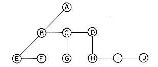
In arriving at the binary tree representation of a tree we shall implicitly make use of the fact that the order of the children of a node is not important. Suppose we have the tree of figure 5.14.
Then, we observe that the reason we needed nodes with many link fields is that the prior representation was based on the parent-child relationship and a node can have any number of children. To obtain a binary tree representation, we need a relationship, between the nodes, that can be characterized by at most two quantities. One such relationship is the leftmost-child-next-right-sibling relationship. Every node has at most one leftmost child and at most one next right sibling. In the tree of figure 5.14, the leftmost child of B is E and the next right sibling of B is C. Strictly speaking, since the order of children in a tree is not important, any of the children of a node could be its leftmost child and any of its siblings could be its next right sibling. For the sake of definiteness, we choose the nodes based upon how the tree is drawn. The binary tree corresponding to the tree of figure 5.14 is thus obtained by connecting together all siblings of a node and deleting all links from a node to its children except for the link to its leftmost child. The node structure corresponds to that of
Using the transformation described above, we obtain the following representation for the tree of figure 5.14.
This does not look like a binary tree, but if we tilt it roughly 45
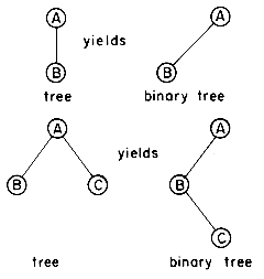
Let us try this transformation on some simple trees just to make sure we've got it.
One thing to notice is that the RCHILD of the root node of every resulting binary tree will be empty. This is because the root of the tree we are transforming has no siblings. On the other hand, if we have a forest then these can all be transformed into a single binary tree by first obtaining the binary tree representation of each of the trees in the forest and then linking all the binary trees together through the SIBLING field of the root nodes. For instance, the forest with three trees
yields the binary tree
We can define this transformation in a formal way as follows:
If T1, ...,Tn is a forest of trees, then the binary tree corresponding to this forest, denoted by B(T1, ..., Tn):
(i) is empty if n = 0;
(ii) has root equal to root (T1); has left subtree equal to B(T11,T12, ...,T1m) where T11, ..., T1m are the subtrees of root(T1); and has right subtree B(T2, ..., Tn).
Preorder and inorder traversals of the corresponding binary tree T of a forest F have a natural correspondence with traversals on F. Preorder traversal of T is equivalent to visiting the nodes of F in tree preorder which is defined by:
(i) if F is empty then return;
(ii) visit the root of the first tree of F;
(iii) traverse the subtrees of the first tree in tree preorder;
(iv) traverse the remaining trees of F in tree preorder.
Inorder traversal of T is equivalent to visiting the nodes of F in tree inorder as defined by:
(i) if F is empty then return;
(ii) traverse the subtrees of the first tree in tree inorder;
(iii) visit the root of the first tree;
(iv) traverse the remaining trees in tree inorder.
The above definitions for forest traversal will be referred to as preorder and inorder. The proofs that preorder and inorder on the corresponding binary tree are the same as preorder and inorder on the forest are left as exercises. There is no natural analog for postorder traversal of the corresponding binary tree of a forest. Nevertheless, we can define the postorder traversal of a forest as:
(i) if F is empty then return;
(ii) traverse the subtrees of the first tree of F in tree postorder;
(iii) traverse the remaining trees of F in tree postorder;
(iv) visit the root of the first tree of F.
This traversal is used later on in section 5.8.3 for describing the minimax procedure.
In this section we study the use of trees in the representation of sets. We shall assume that the elements of the sets are the numbers 1, 2, 3, ..., n. These numbers might, in practice, be indices into a symbol table where the actual names of the elements are stored. We shall assume that the sets being represented are pairwise disjoint; i.e., if Si and Sj, i
(i) Disjoint set union ... if Si and Sj are two disjoint sets, then their union Si
(ii) Find(i) ... find the set containing element i. Thus, 4 is in set S3 and 9 is in set S1.
The sets will be represented by trees. One possible representation for the sets S1, S2 and S3 is:
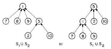
Note that the nodes are linked on the parent relationship, i.e. each node other than the root is linked to its parent. The advantage of this will become apparent when we present the UNION and FIND algorithms. First, to take the union of S1 and S2 we simply make one of the trees a subtree of the other. S1
In order to find the union of two sets, all that has to be done is to set the parent field of one of the roots to the other root. This can be accomplished easily if, with each set name, we keep a pointer to the root of the tree representing that set. If, in addition, each root has a pointer to the set name, then to determine which set an element is currently in, we follow parent links to the root of its tree and use the pointer to the set name. The data representation for S1, S2 and S3 may then take the form:
In presenting the UNION and FIND algorithms we shall ignore the actual set names and just identify sets by the roots of the trees representing them. This will simplify the discussion. The transition to set names is easy. If we determine that element i is in a tree with root j and j has a pointer to entry k in the set name table, then the set name is just NAME(k). If we wish to union sets Si and Sj, then we wish to union the trees with roots POINTER(Si) and POINTER(Sj). As we shall see, in many applications the set name is just the element at the root. The operation of FIND(i) now becomes: determine the root of the tree containing element i. UNION(i,j) requires two trees with roots i and j to be joined. We shall assume that the nodes in the trees are numbered 1 through n so that the node index corresponds to the element index. Thus, element 6 is represented by the node with index 6. Consequently, each node needs only one field: the PARENT field to link to its parent. Root nodes have a PARENT field of zero. Based on the above discussion, our first attempt at arriving at UNION, FIND algorithms would result in the algorithms U and F below.
While these two algorithms are very easy to state, their performance characteristics are not very good. For instance, if we start off with p elements each in a set of its own, i.e., Si = {i}, 1
U(1,2), F(1), U(2,3), F(1), U(3,4)
F(1), U(4,5), ...,F(1), U(n - 1,n)
This sequence results in the degenerate tree:
Since the time taken for a union is constant, all the n - 1 unions can be processed in time O(n). However, each FIND requires following a chain of PARENT links from one to the root. The time required to process a FIND for an element at level i of a tree is O(i). Hence, the total time needed to process the n - 2 finds is
The time required to perform a union has increased somewhat but is still bounded by a constant, i.e. it is O(1). The FIND algorithm remains unchanged. The maximum time to perform a find is determined by Lemma 5.5.
Lemma 5.5: Let T be a tree with n nodes created as a result of algorithm UNION. No node in T has level greater
Proof: The lemma is clearly true for n = 1. Assume it is true for all trees with i nodes, i
Example 5.1 shows that the bound of Lemma 5.5 is achievable for some sequence of unions.
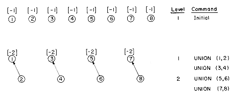
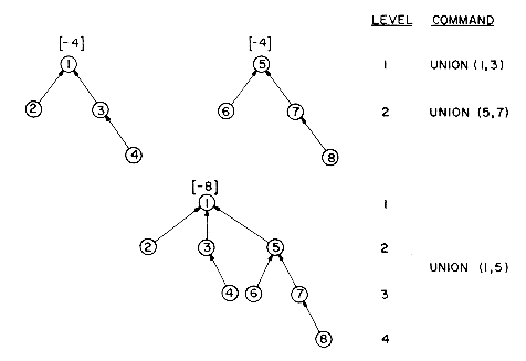
Example 5.1: Consider the behavior of algorithm UNION on the following sequence of unions starting from the initial configuration
PARENT(i) = -COUNT(i) = -1, 1
UNION(1,2), UNION(3,4), UNION(5,6), UNION(7,8),
UNION(1,3), UNION(5,7), UNION(1,5).
The following trees are obtained:
As is evident, the maximum level in any tree is
As a result of Lemma 5.5, the maximum time to process a find is at most O(log n) if there are n elements in a tree. If an intermixed sequence of n - 1 UNION and m FIND operations is to be processed, then the worst case time becomes O(n + m log n). Surprisingly, further improvement is possible. This time the modification will be made in the FIND algorithm using the Collapsing Rule: If j is a node on the path from i to its root and PARENT(j)
This modification roughly doubles the time for an individual find. However, it reduces the worst case time over a sequence of finds.
Example 5.2: : Consider the tree created by algorithm UNION on the sequence of unions of example 5.1. Now process the following 8 finds:
FIND(8), FIND(8), ... FIND(8)
Using the old version F of algorithm FIND, FIND(8) requires going up 3 parent link fields for a total of 24 moves to process all 8 finds. In algorithm FIND, the first FIND(8) requires going up 3 links and then resetting 3 links. Each of the remaining 7 finds requires going up only 1 link field. The total cost is now only 13 moves.
The worst case behavior of the UNION-FIND algorithms while processing a sequence of unions and finds is stated in Lemma 5.6. Before stating this lemma, let us introduce a very slowly growing function
The definition of Ackermann's function used here is:
The function A(p,q) is a very rapidly growing function. One may prove the following three facts:
If we assume m
Lemma 5.6: [Tarjan] Let T(m,n) be the maximum time required to process any intermixed sequence of m
Even though the function
Let us look at an application of algorithms UNION and FIND to processing the equivalence pairs of section 4.6. The equivalence classes to be generated may be regarded as sets. These sets are disjoint as no variable can be in two equivalence classes. To begin with all n variables are in an equivalence class of their own; thus PARENT(i) = -1, 1
In Chapter 6 we shall see another application of the UNION-FIND algorithms.
Example 5.3: We shall use the UNION-FIND algorithms to process the set of equivalence pairs of scction 4.6. Initially, there are 12 trees, one for each variable. PARENT(i) = -1, 1
Each tree represents an equivalence class. It is possible to determine if two elements are currently in the same equivalence class at each stage of the processing by simply making two finds.
Another very useful application of trees is in decision making. Consider the well-known eight coins problem. Given coins a,b,c,d,e,f,g,h, we are told that one is a counterfeit and has a different weight than the others. We want to determine which coin it is, making use of an equal arm balance. We want to do so using a minimum number of comparisons and at the same time determine whether the false coin is heavier or lighter than the rest. The tree below represents a set of decisions by which we can get the answer to our problem. This is why it is called a decision tree. The use of capital H or L means that the counterfeit coin is heavier or lighter. Let us trace through one possible sequence. If a + b + c < d + e + f, then we know that the false coin is present among the six and is neither g nor h. If on our next measurement we find that a + d < b + e, then by interchanging d and b we have no change in the inequality. This tells us two things: (i) that c or f is not the culprit, and (ii) that b or d is also not the culprit. If a + d was equal to b + e, then c or f would be the counterfeit coin. Knowing at this point that either a or e is the counterfeit, we compare a with a good coin, say b. If a = b, then e is heavy, otherwise a must be light.
By looking at this tree we see that all possibilities are covered, since there are 8 coins which can be heavy or light and there are 16 terminal nodes. Every path requires exactly 3 comparisons. Though viewing this problem as a decison tree is very useful it does not immediately give us an algorithm. To solve the 8 coins problem with a program, we must write a series of tests which mirror the structure of the tree. If we try to do this in SPARKS using the if-then-else statement, we see that the program looks like a dish of spaghetti. It is impossible to discern the flow of the program. Actually this type of processing is much more clearly expressed using the case statement.
We will make use of a procedure to do the last comparison.
The procedure EIGHTCOINS appears on the next page. The program is now transparent and clearly mirrors the decision tree of figure 5.16.
Another interesting application of trees is in the playing of games such as tic-tac-toe, chess, nim, kalah, checkers, go, etc. As an example, let us consider the game of nim. This game is played by two players A and B. The game itself is described by a board which initially contains a pile of n toothpicks. The players A and B make moves alternately
with A making the first move. A legal move consists of removing either 1, 2 or 3 of the toothpicks from the pile. However, a player cannot remove more toothpicks than there are on the pile. The player who removes the last toothpick loses the game and the other player wins. The board configuration at any time is completely specified by the number of toothpicks remaining in the pile. At any time the game status is determined by the board configuration together with the player whose turn it is to make the next move. A terminal board cofiguration is one which represents either a win, lose or draw situation. All other configurations are nonterminal. In nim there is only one terminal configuration: there are no toothpicks in the pile. This configuration is a win for player A if B made the last move, otherwise it is a win for B. The game of nim cannot end in a draw.
A sequence C1, ...,Cm of board configurations is said to be valid if:
(i) C1 is the starting configuration of the game;
(ii) Ci, 0 < i < m, are nonterminal configurations;
(iii) Ci+1 is obtained from Ci by a legal move made by player A if i is odd and by player B if i is even. It is assumed that there are only finitely many legal moves.
A valid sequence C1, ...,Cm of board configurations with Cm a terminal configuration is an instance of the game. The length of the sequence C1,C2, ...,Cm is m. A finite game is one in which there are no valid sequences of infinite length. All possible instances of a finite game may be represented by a game tree. The tree of figure 5.17 is the game free for nim with n = 6. Each node of the tree represents a board configuration. The root node represents the starting configuration C1. Transitions from one level to the next are made via a move of A or B. Transitions from an odd level represent moves made by A. All other transitions are the result of moves made by B. Square nodes have been used in figure 5.17 to represent board configurations when it was A's turn to move. Circular nodes have been used for other configurations. The edges from level 1 nodes to level 2 nodes and from level 2 nodes to level 3 nodes have been labeled with the move made by A and B respectively (for example, an edge labeled 1 means 1 toothpick is to be removed). It is easy to figure out the labels for the remaining edges of the tree. Terminal configurations are represented by leaf nodes. Leaf nodes have been labeled by the name of the player who wins when that configuration is reached. By the nature of the game of nim, player A can win only at leaf nodes on odd levels while B can win only at leaf nodes on even levels. The degree of any node in a game tree is at most equal to the number of distinct legal moves. In nim there are at most 3 legal moves from any configuration. By definition, the number of legal moves from any configuration is finite. The depth of a game tree is the length of a longest instance of the game. The depth of the nim tree of figure 5.17 is 7. Hence, from start to finish this game involves at most 6 moves. It is not difficult to see how similar game trees may be constructed for other finite games such as chess, tic-tac-toe, kalah, etc. (Strictly speaking, chess is not a finite game as it is possible to repeat board configurations in the game. We can view chess as a finite game by disallowing this possibility. We could, for instance, define the repetition of a board configuration as resulting in a draw.)
Now that we have seen what a game tree is, the next question is "of what use are they?" Game trees are useful in determining the next move a player should make. Starting at the initial configuration represented by the root of figure 5.17 player A is faced with the choice of making any one of three possible moves. Which one should he make? Assuming that player A wants to win the game, he should make the move that maximizes his chances of winning. For the simple tree of figure 5.17 this move is not too difficult to determine. We can use an evaluation function E(X) which assigns a numeric value to the board configuration X. This function is a measure of the value or worth of configuration X to player A. So, E(X) is high for a configuration from which A has a good chance of winning and low for a configuration from which A has a good chance of losing. E(X) has its maximum value for configurations that are either winning terminal configurations for A or configurations from which A is guaranteed to win regardless of B's countermoves. E(X) has its minimum value for configurations from which B is guaranteed to win.
For a game such as nim with n = 6, whose game tree has very few nodes, it is sufficient to define E(X) only for terminal configurations. We could define E(X) as:
Using this evaluation function we wish to determine which of the configurations b, c, d player A should move the game into. Clearly, the choice is the one whose value is max {V(b), V(c), V(d)} where V(x) is the value of configuration x. For leaf nodes x, V(x) is taken to be E(x). For all other nodes x let d
let c1,c2, ...,cd be the configurations represented by the children of x. Then V(x) is defined by:
The justification for (5.3) is fairly simple. If x is a square node, then it is at an odd level and it will be A's turn to move from here if the game ever reaches this node. Since A wants to win he will move to that child node with maximum value. In case x is a circular node it must be on an even level and if the game ever reaches this node, then it will be B's turn to move. Since B is out to win the game for himself, he will (barring mistakes) make a move that will minimize A's chances of winning. In this case the next configuration will be
For games such as nim with n = 6, the game trees are sufficiently small that it is possible to generate the whole tree. Thus, it is a relatively simple matter to determine whether or not the game has a winning strategy. Moreover, for such games it is possible to make a decision on the next move by looking ahead all the way to terminal configurations. Games of this type are not very interesting since assuming no errors are made by either player, the outcome of the game is predetermined and both players should use similar evaluation functions, i.e., EA(X) = 1 for X a winning configuration and EA(X) = - 1 for X a losing configuration for A; EB(X) = - EA(X).
Of greater interest are games such as chess where the game tree is too large to be generated in its entirety. It is estimated that the game tree for chess has >10100 nodes. Even using a computer which is capable of generating 1011 nodes a second, the complete generation of the game tree for chess would require more than 1080 years. In games with large game trees the decision as to which move to make next can be made only by looking at the game tree for the next few levels. The evaluation function E(X) is used to get the values of the leaf nodes of the subtree generated and then eq. (5.3) can be used to get the values of the remaining nodes and hence to determine the next move. In a game such as chess it may be possible to generate only the next few levels (say 6) of the tree. In such situations both the quality of the resulting game and its outcome will depend upon the quality of the evaluating functions being used by the two players as well as of the algorithm being used to determine V(X) by minimax for the current game configuration. The efficiency of this algorithm will limit the number of nodes of the search tree that can be generated and so will have an effect on the quality of the game.
Let us assume that player A is a computer and attempt to write an algorithm that A can use to compute V(X). It is clear that the procedure to compute V(X) can also be used to determine the next move that A should make. A fairly simple recursive procedure to evaluate V(X) using minimax can be obtained if we recast the definition of minimax into the following form:
where e(X) = E(X) if X is a position from which A is to move and e(X) = - E(X) otherwise.
Starting at a configuration X from which A is to move, one can easily prove that eq. (5.4) computes V'(X) = V(X) as given by eq. (5.3). In fact, values for all nodes on levels from which A is to move are the same as given by eq. (5.3) while values on other levels are the negative of those given by eq. (5.3).
The recursive procedure to evaluate V'(X) based on eq. (5.4) is then VE(X,l). This algorithm evaluates V'(X) by generating only l levels of the game tree beginning with X as root. One may readily verify that this algorithm traverses the desired subtree of the game tree in postorder.
An Initial call to algorithm VE with X = P11 and l = 4 for the hypothetical game of figure 5.18 would result in the generation of the complete game tree. The values of various configurations would be determined in the order: P31, P32, P21, P5l, P52, P53, P41, P54, P55, P56, P42, P33, ...,P37,P24, P11. It is possible to introduce, with relative ease, some heuristics into algorithm VE that will in general result in the generation of only a portion of the possible configurations while still computing V'(X) accurately.
Consider the game tree of figure 5.18. After V(P41) has been computed, it is known that V(P33) is at least V(P41)= 3. Next, when V(P55) is determined to be 2, then we know that V(P42) is at most 2. Since P33 is a max position, V(P42) cannot affect V(P33). Regardless of the values of the remaining children of P42, the value of P33 is not determined by V(P42) as V(P42) cannot be more than V(P41). This observation may be stated more formally as the following rule: The alpha value of a max position is defined to be the minimum possible value for that position. If the value of a min position is determined to be less than or equal to the alpha value of its parent, then we may stop generation of the remaining children of this min position. Termination of node generation under this rule is known as alpha cutoff. Once V(P41) in figure 5.18 is determined, the alpha value of P33 becomes 3. V(P55)
A corresponding rule may be defined for min positions. The beta value of a min position is the maximum possible value for that position. If the value of a max position is determined to be greater than or equal to the beta value of its parent node, then we may stop generation of the remaining children of this max position. Termination of node generation under this rule is called beta cutoff. In figure 5.18, once V(P35) is determined, the beta value of P23 is known to be at most -
In actually introducing alpha-beta pruning into algorithm VE it is necessary to restate this rule in terms of the values defined by eq. (5.4). Under eq. (5.4) all positions are max positions since the values of the min positions of eq. (5.3) have been multiplied by -1. The alpha-beta pruning rule now reduces to the following rule: let the B value of a position be the minimum value that that position can have.
For any position X, let B be the B - value of its parent and let D = -B. Then, if the value of X is determined the greater than or equal to D, we may terminate generation of the remaining children of X. Incorporating this rule into algorithm VE is fairly straightforward and results in algorithm VEB. This algorithm has the additional parameter D which is the negative of the B value of the parent of X.
If Y is a position from which A is to move, then the initial call VEB(Y,l,
One may easily verify that the initial call AB(Y,l, -
Figure 5.19(b) shows a hypothetical game tree in which the use of algorithm AB results in greater pruning than achieved by algorithm VEB. Let us first trace the action of VEB on the tree of figure 5.19(b). We assume the initial call to be VEB(P1,l,
As a conclusion to our chapter on trees, we determine the number of distinct binary trees having n nodes. We know that if n = 0 or n = 1 there is one such tree. If n = 2, then there are two distinct binary trees
and if n = 3, there are five
How many distinct binary trees are there with n nodes?
Before solving this problem let us look at some other counting problems that are equivalent to this one.
In section 5.4 we introduced the notion of preorder, inorder and postorder traversals. Suppose we are given the preorder sequence
A B C D E F G H I
and the inorder sequence
B C A E D G H F I
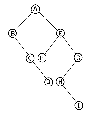
of the same binary tree. Does such a pair of sequences uniquely define a binary tree? Asked another way, can the above pair of sequences come from more than one binary tree. We can construct the binary tree which has these sequences by noticing that the first letter in preorder, A, must be the root and by the definition of inorder all nodes preceding A must occur in the left subtree and the remaining nodes occur in the right subtree.
This gives us
as our first approximation to the correct tree. Moving right in the preorder sequence we find B as the next root and from the inorder we see B has an empty left subtree and C is in its right subtree. This gives
as the next approximation. Continuing in this way we arrive at the binary tree
By formalizing this argument, see the exercises, we can verify that every binary tree has a unique pair of preorder-inorder scquences.
Let the nodes of an n node binary tree be numbered 1 to n. The inorder permutation defined by such a binary tree is the order in which its nodes are visited during an inorder traversal of the tree. A preorder permutation is similarly defined.
As an example, consider the binary tree above with the following numbering of nodes:
Its preorder permutation is 1,2, ...,9 and its inorder permutation is 2,3,1,5,4,7,8,6,9.
If the nodes of a binary tree are numbered such that its preorder permutation is 1,2, ...,n, then from our earlier discussion it follows that distinct binary trees define distinct inorder permutations. The number of distinct binary trees is thus equal to the number of distinct inorder permutations obtainable from binary trees having the preorder permutation 1,2, ...,n.
Using this concept of an inorder permutation, it is possible to show that the number of distinct permutations obtainable by passing the numbers 1 to n through a stack and deleting in all possible ways is equal to the number of distinct binary trees with n nodes (see the exercises). If we start with the numbers 1,2,3 then the possible permutations obtainable by a stack are
1,2,3; 1,3,2; 2,1,3; 3,2,1; 3, 2, 1;
It is not possible to obtain 3,1,2. Each of these five permutations corresponds to one of the five distinct binary trees with 3 nodes
Another problem which surprisingly has connection with the previous two is the following: we have a product of n matrices
M1 * M2 * M3 * ... * Mn
that we wish to compute. We can perform these operations in any order because multiplication of matrices is associative. We ask the question: how many different ways can we perform these multiplications? For example, if n = 3, there are two possibilities
(M1 * M2) * M3 and M1 * (M2 * M3)
and if n = 4, there are five ways
((M1 * M2) * M3) * M4, (M1 * (M2 * M3)) * M4,
M1 * ((M2 * M3) * M4)
(M1 * (M2 * (M3 * M4))), ((M1 * M2) * (M3 * M4))
Let bn be the number of different ways to compute the product of n matrices. Then b2 = 1, b3 = 2, b4 = 5. Let Mij, i
If we can determine an expression for bn only in terms of n, then we have a solution to our problem. Now instead let bn be the number of distinct binary trees with n nodes. Again an expression for bn in terms of n is what we want. Then we see that bn is the sum of all possible binary trees formed in the following way, a root and two subtrees with bi and bn-i-1 nodes,
for 0
This formula and the previous one are essentially the same.
So, the number of binary trees with n nodes, the number of permutations of 1 to n obtainable with a stack, and the number of ways to multiply n + 1 factors are all equal to the same number!
To obtain this number we must solve the recurrence of eq. (5.5). To begin we let
which is the generating function for the number of binary trees. Next, observe that by the recurrence relation we get the identity
x B2(x) = B(x) - 1
Using the formula to solve quadratics and the fact (eq. (5.5)) that B(0) = b0 = 1 we get:
It is not clear at this point that we have made any progress but by using the binomial theorem to expand (1 - 4x)1/2 we get
Comparing eqs. (5.6) and (5.7)we see that bn which is the coefficient of xn in B(x) is:
Some simplification yields the more compact form
which is approximately
bn= O(4n/n3/2)
For other representations of trees see
The Art of Computer Programming: Fundamental Algorithms, by D. Knuth, second edition, Addison-Wesley, Reading, 1973.
For the use of trees in generating optimal compiled code see
"The generation of optimal code for arithmetic expressions'' by R. Sethi and J. Ullman, JACM, vol. 17, no. 4, October 1970, pp. 715-728.
"The generation of optimal code for a stack machine'' by J. L. Bruno and T. Lassagne, JACM, vol. 22, no. 3, July 1975, pp. 382-396.
Algorithm INORDER4 of the exercises is adapted from
"An improved algorithm for traversing binary trees without auxiliary stack," by J. Robson, Information Processing Letters, vol. 2, no. 1, March 1973, p. 12-14.
Further tree traversal algorithms may be found in:
''Scanning list structures without stacks and tag bits,'' by G. Lindstrom, Information Processing Letters, vol. 2, no. 2, June 1973, p. 47-51.
"Simple algorithms for traversing a tree without an auxiliary stack,'' by B. Dwyer, Information Processing Letters, vol. 2, no. 5, Dec. 1973, p. 143-145.
The use of threads in conneetion with binary trees is given in
"Symbol manipulation by threaded lists,'' by A. Perlis and C. Thornton, CACM, vol. 3, no. 4, April 1960, pp. 195-204.
For a further analysis of the set representation problem see
The Design and Analysis of Computer A1gorithms, A. Aho, J. Hopcroft and J. Ullman, Addison-Wesley, Reading, 1974.
The computing time analysis of the UNION-FIND algorithms may be found in:
"Efficiency of a good but not linear set union algorithm" by R. Tarjan, JACM, vol. 22, no. 2, April 1975, pp. 215-225.
Our discussion of alpha-beta cutoffs is from
"An analysis of alpha beta cutoffs" by D. Knuth, Stanford Technical Report 74-441, Stanford University, 1975.
For more on game playing see
Problem Solving Methods in Artificial Intelligence by N. Nilsson, McGraw-Hill, New York, 1971.
Artificial Intelligence: The Heuristic Programming Approach by J. Slagle, McGraw-Hill, New York, 1971.
1. For the binary tree below list the terminal nodes, the nonterminal nodes and the level of each node.
2. Draw the internal memory representation of the above binary tree using (a) sequential, (b) linked, and (c) threaded linked representations.
3. Write a procedure which reads in a tree represented as a list as in section 5.1 and creates its internal representation using nodes with 3 fields, TAG, DATA, LINK.
4. Write a procedure which reverses the above process and takes a pointer to a tree and prints out its list representation.
5. Write a nonrecursive version of procedure PREORDER.
6. Write a nonrecursive version of procedure POSTORDER without using go to's.
7. Rework INORDER3 so it is as fast as possible. (Hint: minimize the stacking and the testing within the loop.)
8. Write a nonrecursive version of procedure POSTORDER using only a fixed amount of additional space. (See exercise 36 for details)
9. Do exercise 8 for the case of PREORDER.
10. Given a tree of names constructed as described in section 5.5 prove that an inorder traversal will always print the names in alphabetical order.
Exercises 11-13 assume a linked representation for a binary tree.
11. Write an algorithm to list the DATA fields of the nodes of a binary tree T by level. Within levels nodes are to be listed left to right.
12. Give an algorithm to count the number of leaf nodes in a binary tree T. What is its computing time?
13. Write an algorithm SWAPTREE(T) which takes a binary tree and swaps the left and right children of every node. For example, if T is the binary tree
14. Devise an external representation for formulas in the propositional calculus. Write a procedure which reads such a formula and creates a binary tree representation of it. How efficient is your procedure?
15. Procedure POSTORDER-EVAL must be able to distinguish between the symbols
16. What is the computing time for POSTORDER-EVAL? First determine the logical parameters.
17. Write an algorithm which inserts a new node T as the left child of node S in a threaded binary tree. The left pointer of S becomes the left pointer of T.
18. Write a procedure which traverses a threaded binary tree in postorder. What is the time and space requirements of your method?
19. Define the inverse transformation of the one which creates the associated binary tree from a forest. Are these transformations unique?
20. Prove that preorder traversal on trees and preorder traversal on the associated binary tree gives the same result.
21. Prove that inorder traversal for trees and inorder traversal on the associated binary tree give the same result.
22. Using the result of example 5. 3, draw the trees after processing the instruction UNION(12,10).
23. Consider the hypothetical game tree:
(a) Using the minimax technique (eq. (5.3)) obtain the value of the root node .
(b) What move should player A make?
(c) List the nodes of this game tree in the order in which their value is computed by algorithm VE.
(d) Using eq. (5.4) compute V' (X) for every node X in the tree.
(e) Which nodes of this tree are not evaluated during the computation of the value of the root node using algorithm AB with X = root, l=
24. Show that V'(X) computed by eq. (5.4) is the same as V(X) computed by eq. (5.3) for all nodes on levels from which A is to move. For all other nodes show that V(X) computed by eq. (5.3) is the negative of V'(X) computed by eq. (5.4).
25. Show that algorithm AB when initially called with LB = -
26. Prove that every binary tree is uniquely defined by its preorder and inorder sequences .
27. Do the inorder and postorder sequences of a binary tree uniquely define the binary tree? Prove your answer.
28. Answer exercise 27 for preorder and postorder.
29. Write an algorithm to construct the binary tree with a given preorder and inorder sequence.
30. Do exercise 29 for inorder and postorder.
31. Prove that the number of distinct permutations of 1,2, ...,n obtainable by a stack is equal to the number of distinct binary trees with n nodes. (Hint: Use the concept of an inorder permutation of a tree with preorder permutation 1,2, ...,n).
32. Using Stirling's formula derive the more accurate value of the number of binary trees with n nodes,
33. Consider threading a binary tree using preorder threads rather than inorder threads as in the text. Is it possible to traverse a binary tree in preorder without a stack using these threads?
34. Write an algorithm for traversing an inorder threaded binalry tree in preorder.
35. The operation PREORD(btree)
Devise similar axioms for INORDER AND POSTORDER.
36. The algorithm on page 281 performs an inorder traversal without using threads, a stack or a PARENT field. Verify that the algorithm is correct by running it on a variety of binary trees which cause every statement to execute at least once. Before attempting to study this algorithm be sure you understand MARK2 of section 4.10.
37. Extend the equivalence algorithm discussed in section 5.8.1 so it handles the equivalencing of arrays (see section 4.6). Analyze the computing time of your solution.
38. [Wilczynski] Following the conventions of LISP assume nodes with two fields
a) Give a sequence of HEAD, TAIL operations for extracting a from the lists: ((cat)), ((a)), (mart), (((cb))a).
b) Write recursive procedures for: COPY, REVERSE, APPEND.
c) Implement this "LISP" subsystem. Store atoms in an array, write procedures MAKELIST and LISTPRINT for input and output of lists.
 0 disjoint trees. The notion of a forest is very close to that of a tree because if we remove the root of a tree we get a forest. For example, in figure 5.2 if we remove A we get a forest with three trees.
 _____________________________________
| | | | | |
|DATA |LINK 1 |LINK 2|


 |LINK n |
 |______|________|______|______|_______|

List representation for the tree of figure 5.2
5.2 BINARY TREES
structure BTREE
declare CREATE( )
 btree
btreeISMTBT(btree)
 boolean
MAKEBT(btree,item,btree)
 btree
btreeLCHILD(btree)
 btree
btreeDATA(btree)
 item
itemRCHILD(btree)
 btree
btreefor all p,r
 btree, d
  item let
ISMTBT(CREATE) :: = true
ISMTBT(MAKEBT(p,d,r)) :: = false
LCHILD(MAKEBT(p,d,r)):: = p; LCHILD(CREATE):: = error
DATA(MAKEBT(p,d,r)) :: = d; DATA(CREATE) :: = error
RCHILD(MAKEBT(p,d,r)) :: = r; RCHILD(CREATE) :: = error
end
end BTREE

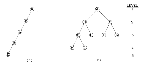
Figure 5.3 Two Sample Binary Trees
 1 and
1 and 1.
1. = 2i - 1.
 j < i, the maximum number of nodes on level j is 2j - 1.
 (maximum number of nodes on level i)
 2 we have:
(5.1)
(5.2)
5.3 BINARY TREE REPRESENTATIONS
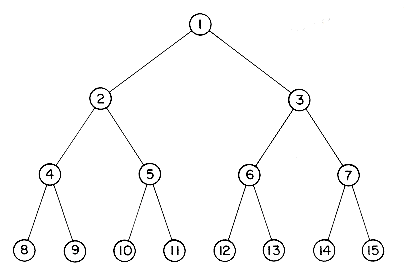
Figure 5.4 Full Binary Tree of Depth 4 with Sequential Node Numbers
 i
i  n we have:
 1. When i = 1, i is the root and has no parent.
 n. If 2i > n, then i has no left child.
 n. If 2i + 1 > n, then i has no right child.
 j
j  i, LCHILD(j) is at 2j. Then, the two nodes immediately preceding LCHILD (i + 1) in the representation are the right child of i and the left child of i. The left child of i is at 2i. Hence, the left child of i + 1 is at 2i + 2 = 2(i + 1) unless 2(i + 1) > n in which case i + 1 has no left child.
 TREE TREE
----- -----
(1) | A | | A |
|-----| |-----|
(2) | B | | B |
|-----| |-----|
(3) | - | | C |
|-----| |-----|
(4) | C | | D |
|-----| |-----|
(5) | - | | E |
|-----| |-----|
(6) | - | | F |
|-----| |-----|
(7) | - | | G |
|-----| |-----|
(8) | D | | H |
|-----| |-----|
(9) | - | | I |
|-----| -----
. | . |
|-----|
. | . |
|-----|
. | . |
|-----|
(16) | E |
-----
Figure 5.5 Array Representation of the Binary Trees of Figure 5.3

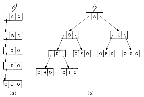
Figure 5.6 Linked Representation for the Binary Trees of Figure 5.3.
5.4 BINARY TREE TRAVERSAL
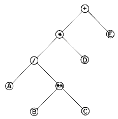
Figure 5.7 Binary Tree with Arithmetic Expression
procedure INORDER(T)
//T is a binary tree where each node has three fields L-
CHILD,DATA,RCHILD//
if T
 0 then [call INORDER(LCHILD(T))
print(DATA(T))
call(INORDER(RCHILD(T))]
end INORDER
Call of value
INORDER in root Action
------- ------- ----------
MAIN +
1 *
2 /
3 A
4 0 print('A') 4 0 print('/') 3 **
4 B
5 0 print('B') 5 0 print('**') 4 C
5 0 print('C') 5 0 print('*') 2 D
3 0 print('D') 3 0 print('+') 1 E
2 0 print('E') 2 0
procedure PREORDER (T)
//T is a binary tree where each node has three fields L-
CHILD,DATA,RCHILD//
if T
 0 then [print (DATA(T))
call PREORDER(LCHILD(T))
call PREORDER(RCHILD(T))]]
end PREORDER
procedure POSTORDER (T)
//T is a binary tree where each node has three fields L-
CHILD,DATA,RCHILD//
if T
 0 then [call POSTORDER(LCHILD(T))
call POSTORDER(RCHILD(T))
print (DATA(T))]
end POSTORDER
procedure INORDER1(T)
//a nonrecursive version using a stack of size n//
i
 0 //initialize the stack//
L1: if T
 0 then [i
  i + 2; if i > n then call STACK_FULL
STACK (i - 1)
 T; STACK(i)
  'L2'
'L2'T
 LCHILD(T); go to L1; //traverse left
subtree//
L2: print (DATA(T))
i
 i + 2; if i > n then call STACK--FULL
STACK (i - 1)
 T; STACK(i)
  'L3'
'L3'T
 RCHILD(T); go to L1] //traverse right
subtree//
L3: if i
 0 then [//stack not empty, simulate a return//
T
 STACK (i - 1); X
  STACK (i)
i
 i - 2; go to X]
end INORDER 1
procedure INORDER 2(T)
//a simplified, nonrecursive version using a stack of size n//
i
 0 //initialize stack//
L1: if T
 0 then [i
  i + 1; if i > n then call STACK__FULL
STACK (i)
 T; T
T; T  LCHILD(T); go to L1
L2: print (DATA(T))
T
 RCHILD(T); go to L1]
if i
 0 then [//stack not empty//
T
 STACK (i): i
  i - 1; go to L2]
end INORDER2
procedure INORDER3(T)
//a nonrecursive, no go to version using a stack of size n//
i
 0 //initialize stack//
loop
while T
 0 do //move down LCHILD fields//
i
 i + 1; if i > n then call STACK--FULL
STACK (i)
 T; T
T; T  LCHILD(T)
end
if i = 0 then return
T
 STACK (i); i
  i - 1
i - 1print(DATA(T)); T
 RCHILD(T)
forever
end INORDER3
 T and T
  STACK(i) are executed n times. Moreover, T will equal zero once for every zero link in the tree which is exactly
5.5 MORE ON BINARY TREES
procedure COPY(T)
//for a binary tree T, COPY returns a pointer to an exact copy of
T; new nodes are gotten using the usual mechanism//
Q
 0
0if T
 0 then [R
  COPY(LCHILD(T)) //copy left subtree//
S
 COPY(RCHILD(T)) //copy right subtree//
call GETNODE(Q)
LCHILD(Q)
 R; RCHILD(Q)
  S
S//store in fields of Q//
DATA(Q)
 DATA(T)]
return(Q) //copy is a function//
end COPY
procedure EQUAL(S,T)
//This procedure has value false if the binary trees S and T are not
equivalent. Otherwise, its value is true//
ans
 false
falsecase
: S = 0 and T = 0: ans
 true
true: S
 0 and T
  0:
0:if DATA(S) = DATA(T)
then [ans
 EQUAL(LCHILD(S),LCHILD(T))
if ans then ans
 EQUAL(RCHILD(S),RCHILD(T))]
end
return (ans)
end EQUAL
 (and),
  (or) and
  (not). These variables can only hold one of two possible values, true or false. The set of expressions which can be formed using these variables and operators is defined by the rules: (i) a variable is an expression, (ii) if x,y are expressions then x
  y, x
y, x  y,
y,  x are expressions. Parentheses can be used to alter the normal order of evaluation which is not before and before or. This comprises the formulas in the propositional calculus (other operations such as implication can be expressed using
  ,
,  ,
,  ). The expression
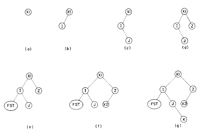
Figure 5.8 Tree of Identifiers
 (x2
(x2 
 x3)
x3)false
 (true
(true 
 false)
= false
 true
true= true

 x2)
x2)  (
( x1
x1  x3)
x3) 
 x3
x3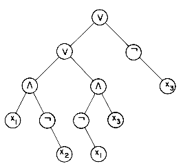
Figure 5.9 Propositional Formula in a Binary Tree

 x2
x2 
 x1
x1  x3
x3 
 x3, the infix form of the expression. The most obvious algorithm to determine satisfiability is to let (x1,x2,x3) take on all possible combinations of truth and falsity and to check the formula for each combination. For n variables there are 2n possible combinations of true = t and false = f, e.g. for n = 3 (t,t,t), (t,t,f), (t,f, t), (t,f,f), (f,t,t), (f,t,f), (f,f,t), (f,f,f). The algorithm will take at least O(g2n) or exponential time where g is the time to substitute values for x1,x2,x3 and evaluate the expression.
 x2 and
  x1
x1  x3 will already be available to us and we can apply the rule for or. Notice that a node containing
  has only a single right branch since not is a unary operator.
 _____________________________
| | | | |
|LCHILD | DATA | VAL | RCHILD |
|_______|______|_____|________|
for all 2n possible combinations do
generate the next combination;
store it in DEF(1) to DEF(n);
call POSTORDER and evaluate T;
if VAL(T) = true then [print DEF(1) to DEF(n)
stop]
end
print ('no satisfiable combination')procedure POSTORDER_EVAL(T)
//a binary tree T containing a propositional formula is evaluated with
the result stored in the VAL field of each node//
if T
 0 then[ call POSTORDER_EVAL(LCHILD(T))
call POSTORDER_EVAL(RCHILD(T))
case
:DATA(T) = '
 : VAL(T)
  not VAL(RCHILD(T))
:DATA(T) = '
 : VAL(T)
  VAL(LCHILD(T) or
VAL(RCHILD(T))
:DATA(T) = '
 : VAL(T)
  VAL(LCHILD(T) and
VAL(RCHILD(T))
:else: VAL(T)
 DEF(DATA(T))
end]
end POSTORDER_EVAL
5.6 THREADED BINARY TREES
LBIT(P) =1 if LCHILD(P) is a normal pointer
LBIT(P) = 0 if LCHILD(P) is a thread
RBIT(P) = 1 if RCHILD(P) is a normal pointer
RBIT(P) = 0 if RCHILD(P) is a thread
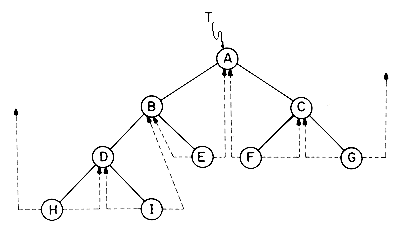
Figure 5.10 Threaded Tree Corresponding to Figure 5.3(b)

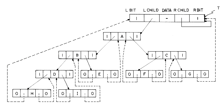
Figure 5.11 Memory Representation of Threaded Tree
procedure INSUC(X)
//find the inorder succcesor of X in a threaded binary tree//
S
 RCHILD(X) //if RBIT(X) = 0 we are done//
if RBIT(X) = 1 then [while LBIT(S) = 1 do //follow left//
S
 LCHILD(S) //until a thread//
end]
return (S)
end INSUC
procedure TINORDER (T)
//traverse the threaded binary tree, T, in inorder//
HEAD
 T
Tloop
T
 INSUC(T)
if T = HEAD then return
print(DATA(T))
forever
end TINORDER
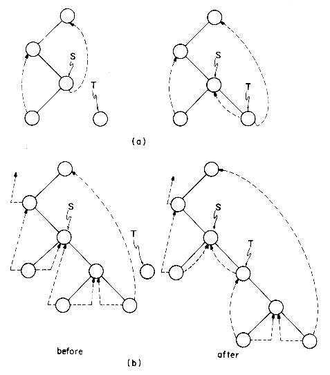
Figure 5.12 Insertion of T as a Right Child of S in a Threaded Binary Tree
procedure INSERT_RIGHT (S,T)
//insert node T as the right child of S in a threaded binary tree//
RCHILD(T)
 RCHILD(S); RBIT(T)
  RBIT(S)
LCHILD(T)
 S; LBIT(T)
  0 //LCHILD(T) is a thread//
RCHILD(S)
 T; RBIT(S)
  1 //attach node T to S//
if RBIT (T) = 1 then [W
 INSUC(T)//S had a right child//
LCHILD(W)
 T]
T]end INSERT_RIGHT
5.7 BINARY TREE REPRESENTATION OF TREES
 1.
1.
Figure 5.13 Possible Node Structure for a k-ary Tree
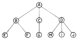
Figure 5.14 A Sample Tree
___________________
| DATA |
|-------------------|
| CHILD | SIBLING |
|_________|_________|
 clockwise we get
Figure 5.15 Associated Binary Tree for Tree of Figure 5.14

5.8 APPLICATIONS OF TREES
5.8.1 Set Representation
 j, are two sets then there is no element which is in both Si and Sj. For example, if we have 10 elements numbered 1 through 10, they may be partitioned into three disjoint sets S1 = {1, 7, 8, 9}; S2= {2, 5, 10} and S3 = {3, 4, 6}. The operations we wish to perform on these sets are:
 Sj = {all elements x such that x is in Si or Sj}. Thus, S1
  S2 = {1, 7, 8, 9, 2, 5, 10}. Since we have assumed that all sets are disjoint, following the union of Si and Sj we can assume that the sets Si and Sj no longer exist independently, i.e., they are replaced by Si
  Sj in the collection of sets.
 S2 could then have one of the following representations

procedure U(i,j)
//replace the disjoint sets with roots i and j, i
 j with their union//
PARENT(i)
 j
jend U
procedure F(i)
//find the root j of the tree containing element i//
j
 i
iwhile PARENT(j) > 0 do //PARENT (j) = 0 if this node is a
root//
j
 PARENT(j)
end
return(j)
end F
 i
i  p, then the initial configuration consists of a forest with p nodes and PARENT(i) = 0, 1
  i
i  p. Now let us process the following sequence of UNION-FIND operations.
 . It is easy to see that this example represents the worst case behavior of the UNION-FIND algorithms. We can do much better if care is taken to avoid the creation of degenerate trees. In order to accomplish this we shall make use of a Weighting Rule for UNION (i,j). If the number of nodes in tree i is less than the number in tree j, then make j the parent of i, otherwise make i the parent of j. Using this rule on the sequence of set unions given before we obtain the trees on page 252. Remember that the arguments of UNION must both be roots. The time required to process all the n finds is only O(n) since in this case the maximum level of any node is 2. This, however, is not the worst case. In Lemma 5.5 we show that using the weighting rule, the maximum level for any node is
  log n
log n  + 1. First, let us see how easy it is to implement the weighting rule. We need to know how many nodes there are in any tree. To do this easily, we maintain a count field in the root of every tree. If i is a root node, then COUNT (i) = number of nodes in that tree. The count can be maintained in the PARENT field as a negative number. This is equivalent to using a one bit field to distinguish a count from a pointer. No confusion is created as for all other nodes the PARENT is positive.
Trees obtained using the weighting rule
procedure UNION(i,j)
//union sets with roots i and j, i
 j, using the weighting rule. PARENT
(i) = - COUNT(i) and PARENT(j) = - COUNT(j)//
x
 PARENT (i) + PARENT(j)
if PARENT(i) > PARENT(j)
then [PARENT (i)
 j //i has fewer nodes//
PARENT (j)
 x]
x]else [PARENT (j)
 i //j has fewer nodes//
PARENT (i)
 x]
x]end UNION
 log2 n
 + 1.
+ 1. n - 1. We shall show that it is also true for i = n. Let T be a tree with n nodes created by the UNION algorithm. Consider the last union operation performed, UNION(k,j). Let m be the number of nodes in tree j and n - m the number in k. Without loss of generality we may assume 1
  m
m  n/2. Then the maximum level of any node in T is either the same as that in k or is one more than that in j. If the former is the case, then the maximum level in T is
 log2 (n - m)
 + 1
+ 1 
 log2 n
 + 1. If the latter is the case then the maximum level in T is
 log2 m
 + 2
+ 2 
 log2 n/2
 + 2.
+ 2. 
 log2 n
 + 1.
+ 1.  i
i  n = 23
 log2 m
 + 1 if the tree has m nodes.
  root(i) then set PARENT(j)
  root(i). The new algorithm then becomes:
procedure FIND(i)
//find the root of the tree containing element i. Use the collapsing
rule to collapse all nodes from i to the root j//
j
 i
iwhile PARENT(j) > 0 do //find root//
j
 PARENT(j)
end
k
 i
iwhile k
 j do //collapse nodes from i to root j//
t
 PARENT(k)
PARENT(k)
 j
jk
 t
tend
return(j)
end FIND
 (m,n) which is related to a functional inverse of Ackermann's function A(p,q). We have the following definition for
  (m,n):
 (m,n) = min{z
  1
1  A(z,4
A(z,4 m/n
m/n ) > log2n}

 0 then (b) and (c) together with the definition of
  (m,n) imply that
  (m,n)
(m,n)  3 for log2n < A(3,4). But from (a), A(3,4) is a very large number indeed! In Lemma 5.6 n will be the number of UNlONs performed. For all practical purposes we may assume log2n < A(3,4) and hence
  (m,n)
(m,n)  3.
3. n FINDs and n - 1 UNIONs. Then k1m
 (m,n)
(m,n)  T(m,n)
  k2m
k2m (m,n) for some positive constants k1 and k2.
  (m,n) is a very slowly growing function, the complexity of UNION-FIND is not linear in m, the number of FINDs. As far as the space requirements are concerned, the space needed is one node for each element.
 i
i  n. If an equivalence pair, i
  j, is to be processed, we must first determine the sets containing i and j. If these are different, then the two sets are to be replaced by their union. If the two sets are the same, then nothing is to be done as the relation i
  j is redundant; i and j are already in the same equivalence class. To process each equivalence pair we need to perform at most two finds and one union. Thus, if we have n variables and m
  n equivalence pairs, the total processing time is at most O(m
 (2m,m)). While for very large n this is slightly worse than the algorithm of section 4.6, it has the advantage of needing less space and also of being "on line."
 i
i  12.
12.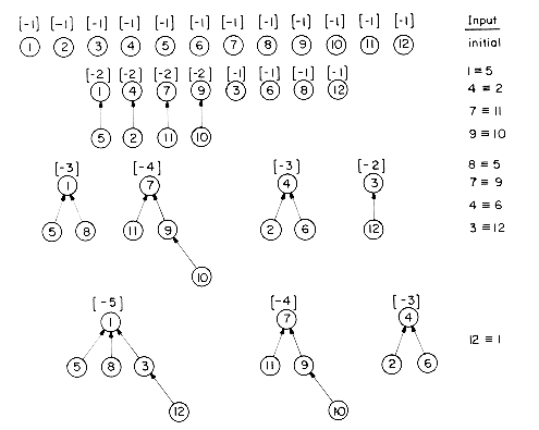
5.8.2 Decision Trees
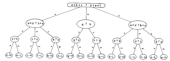
Figure 5.16 Eight Coins Decision Tree
procedure COMP(x,y,z)
//x is compared against the standard coin z//
if x > z then print (x 'heavy')
else print (y 'light')
end COMP
5.8.3 Game Trees
procedure EIGHTCOINS
//eight weights are input; the different one is discovered using only
3 comparisons//
read (a, b, c, d, e, f, g, h)
case
: a + b + c = d + e + f : if g > h then call COMP(g,h,a)
else call COMP(h,g,a)
: a + b + c > d + e + f : case
: a + d = b + e: call COMP(c,f,a)
: a + d > b + e: call COMP(a,e,b)
: a + d < b + e: call COMP(b,d,a)
end
: a + b + c < d + e + f : case
: a + d = b + e: call COMP(f,c,a)
: a + d > b + e: call COMP(d,b,a)
: a + d < b + e: call COMP(e,a,b)
end
end
end EIGHTCOINS
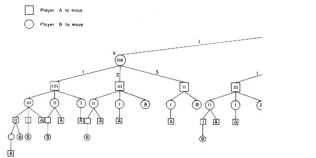
Figure 5.17 Complete Game Tree for Nim with n = 6

 1 be the degree of x and

(5.3)
 {V(ci)}. Equation (5.3) defines the minimax procedure to determine the value of a configuration x. This is illustrated on the hypothetical game of figure 5.18. P11 represents an arbitrary board configuration from which A has to make a move. The values of the leaf nodes are obtained by evaluating the function E(x). The value of P11 is obtained by starting at the nodes on level 4 and computing their values using eq. (5.3). Since level 4 is a level with circular nodes all unknown values on this level may be obtained by taking the minimum of the children values. Next, values on levels 3, 2 and 1 may be computed in that order. The resulting value for P11 is 3. This means that starting from P11 the best A can hope to do is reach a configuration of value 3. Even though some nodes have value greater than 3, these nodes will not be reached, as B's countermoves will prevent the game from reaching any such configuration (assuming B's countermoves are optimal for B with respect to A's evaluation function). For example, if A made a move to P21, hoping to win the game at P31, A would indeed be surprised by B's countermove to P32 resulting in a loss to A. Given A's evaluation function and the game tree of figure 5.18, the best move for A to make is to configuration P22. Having made this move, the game may still not reach configuration P52 as B would, in general, be using a different evaluation function, which might give different values to various board configurations. In any case, the minimax procedure can be used to determine the best move a player can make given his evaluation function. Using the minimax procedure on the game tree for nim (figure 5.17) we see that the value of the root node is V(a) = 1. Since E(X) for this game was defined to be 1 iff A was guaranteed to win, this means that if A makes the optimal move from node a then no matter what B's countermoves A will win. The optimal move is to node b. One may readily verify that from b A can win the game independent of B's countermove!
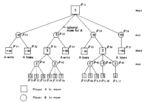
Figure 5.18 Portion of Game Tree for a Hypothetical Game. The value of terminal nodes is obtained from the evaluation function E(x) for player A.

(5.4)
procedure VE(X,l)
//compute V'(X) by looking at most l moves ahead. e(X) is the
evaluation function for player A. For convenience, it is assumed
that starting from any board configuration X the legal moves of
the game permit a transition only to the configurations C1,C2, ...,Cd
if X is not a terminal configuration.//
if X is terminal or l = 0 then return e(X)
ans
 - VE(C1,l - 1 //traverse the first subtree//
for i
 2 to d do //traverse the remaining subtrees//
ans
 max {ans, - VE(Ci, l - 1)}
end
return (ans)
end VE
 alpha value of P33 implies that P56 need not be generated.
 . Generation of P57, P58, P59 gives V(P43) = 0. Thus, V(P43) is greater than or equal to the beta value of P23 and we may terminate the generation of the remaining children of P36. The two rules stated above may be combined together to get what is known as alpha-beta pruning. When alpha-beta pruning is used on figure 5.18, the subtree with root P36 is not generated at all! This is because when the value of P23 is being determined the alpha value of P11 is 3. V(P35) is less than the alpha value of P11 and so an alpha cutoff takes place. It should be emphasized that the alpha or beta value of a node is a dynamic quantity. Its value at any time during the game tree generation depends upon which nodes have so far been generated and evaluated.
procedure VEB(X,l,D)
//determine V'(X) as in eq. (5.4) using the B-rule and looking
only l moves ahead. Remaining assumptions and notation are
the same as for algorithm VE.//
if X is terminal or l = 0 then return e(x)
ans
 -
- . //current lower bound on V'(x)//
for i
 l to d do
ans
 max {ans, - VEB(Ci,l-1,-ans)}
if ans
 D then return (ans) //use B-rule//
end
return (ans)
end VEB
 ) correctly computes V' (Y) with an l move look ahead. Further pruning of the game tree may be achieved by realizing that the B - value of a node X places a lower bound on the value grandchildren of X must have in order to affect X's value. Consider the subtree of figure 5.19(a). If V' (GC(X))
  B then V' (C(X))
  -B. Following the evaluation of C(X), the B-value of X is max{B,-V' (C(X))} = B as V'(C(X))
  -B. Hence unless V' (GC(X)) > B, it cannot affect V' (X) and so B is a lower bound on the value GC(X) should have. Incorporating this lowerbound into algorithm VEB yields algorithm AB. The additional parameter LB is a lowerbound on the value X should have.
procedure AB(X,l,LB,D)
//same as algorithm VEB. LB is a lowerbound on V' (X)//
if X is terminal or l = 0 then return e(X)
ans
 LB //current lowerbound on V' (X)//
for i
 1 to d do
ans
 max{ans,-AB(Ci,l-1,-D,-ans)}
if ans
 D then return (ans)
end
return (ans)
end AB.
 ,
, ) gives the same result as the call VE(Y,l).
 ) where l is the depth of the tree. After examining the left subtree of P1, the B value of P1 is set to 10 and nodes P3, P4, P5 and P6 are generated. Following this, V' (P6) is determined to be 9 and then the B-value of P5 becomes -9. Using this, we continue to evaluate the node P7. In the case of AB however, since the B-value of P1 is 10, the lowerbound for P4 is 10 and so the effective B-value of P4 becomes 10. As a result the node P7 is not generated since no matter what its value V' (P5)
  -9 and this will not enable V' (P4) to reach its lower bound.
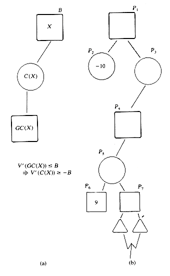
Figure 5.19 Game trees showing lower bounding
5.9 COUNTING BINARY TREES


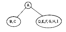

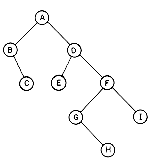


 j, be the product Mi * Mi+1 * ... * Mj. The product we wish to compute is M1n.M1n may be computed by computing any one of the products M1i * Mi+1,n, 1
  i < n. The number of ways to obtain M1i and Mi+1,n is bi and bn-i respectively. Therefore, letting b1 = 1 we have:
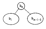
 i
i  n - 1. This says that
(5.5)

(5.6)


(5.7)


REFERENCES
EXERCISES

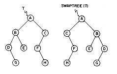
 ,
, ,
,  and a pointer in the DATA field of a node. How should this be done?
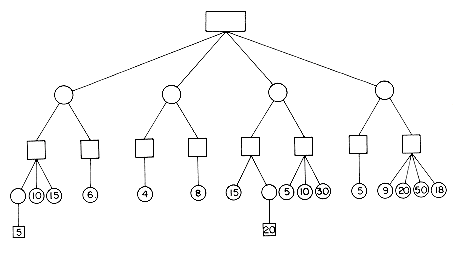
 , LB = -
 and D =
  ?
? and D =
 yields the same results as VE does for the same X and l.
 queue returns a queue whose elements are the data items of btree in preorder. Using the operation APPENDQ(queue, queue)
  queue which concatenates two queues, PREORD can be axiomatized by
PREORD(CREATE) :: = MTQ
PREORD(MAKBT(p,d,r)) :: =
APPENDQ(APPENDQ(ADDQ(MTQ,d),(PREORD(p)),PREORD(r))
 . If A = ((a(bc))) then HEAD(A) = (a(bc)), TAIL(A) = NIL, HEAD(HEAD(A)) = a, TAIL(HEAD(A)) = ((bc)). CONS(A,B) gets a new node T, stores A in its HEAD, B in its TAIL and returns T. B must always be a list. If L = a, M = (bc) then CONS(L,M) = (abc), CONS(M,M) = ((bc)bc). Three other useful functions are: ATOM(X) which is true if X is an atom else false, NULL(X) which is true if X is NIL else false, EQUAL(X,Y) which is true if X and Y are the same atoms or equivalent lists else false.
line procedure INORDER4(T)
//inorder traversal of binary tree T using a fixed amount of
additional storage//
1 if T = 0 then return //empty binary tree//
2 top
 last_right
  0; p
0; p  q
q  T //initialize//
3 loop
4 loop //move down as far as possible//
5 case
6 :LCHILD(p) = 0 and RCHILD(p) = 0:
//can't move down//
7 print (DATA(p)); exit
8 :LCHILD(p) = 0: //move to RCHILD(p)//
9 print(DATA(p)) //visit p//
10 r
 RCHILD(p); RCHILD(p)
  q;
q;q
 p;p
p;p  r
r11 :else: //move to LCHILD(p)//
12 r
 LCHILD(p); LCHILD(p)
  q; q
q; q  p;
p;p
 r
r13 end
14 forever
//p is a leaf node, move upwards to a node whose right
subtree hasn't yet been examined//
15 av
 p //leaf node to be used in stack//
16 loop //move up from p//
17 case
18 :p = T: return //can't move up from root//
19 :LCHILD(q) = 0: //q is linked via RCHILD//
20 r
 RCHILD(q); RCHILD(q)
  p; p
p; p  q; q
q; q  r
r21 :RCHILD(q) = 0: //q is linked via LCHILD//
22 r
 LCHILD(q); LCHILD(q)
  p; p
p; p  q; q
q; q  r;
r;print(DATA(p))
23 :else: //check if p is RCHILD of q//
24 if q = last_right then [//p is RCHILD of q//
25 r
 top; last--right
  LCHILD(r) //update
 last--right//
26 top
 RCHILD(r); //unstack//
27 LCHILD(r)
 RCHILD(r)
  0 //reset leaf
 node links//
28 r
 RCHILD(q); RCHILD(q)
  p; p
p; p  q; q
q; q  r]
r]29 else [//p is LCHILD of q//
30 print (DATA(q)) //visit q//
31 LCHILD(av)
 last_right; RCHILD(av)
  top;
top;top
 av
av32 last_right
 q
q33 r
 LCHILD(q); LCHILD(q)
  p
p//restore link to p//
34 r1
 RCHILD(q); RCHILD(q)
  r; p
r; p  r1; exit
//move right//]
35 end
36 forever
37 forever
38 end INORDER4


