The list is a commonly used data structure and can certainly be incorporated into programming. Lists are so general, common, and useful that even restricted forms of lists are major topics and are the basis for the two chapters that follow this one.
3.1 The List as a Structure
A data structure is many things, including an abstraction. In particular, it is a combination of allocated storage with a set of operations performed on it. The feature that best characterizes structure LIST is that its cells are linked together. Some idea of the nature of structure LIST can be gained by contrasting it with data structure ARRAY. The contrast is related to operations performed on instances of both structures.
The operations applied to lists differ significantly from those applied to arrays.
The list that forms a class roll usually exists, even if there are no names on it, which is true before registration or if everyone drops the course. It defines the roll, empty or not. A list is normally created empty, with no storage occupied by list entries. It may be necessary to allocate space for the list to grow into, just as a piece of paper is reserved for a shopping list; but it may also be possible to avoid the allocation of space before it is needed. In either case, the list itself is initially null (empty), as opposed to an array that is not yet initialized but consists of cells that contain some value.
A list is not only created null, it can become null through the removal of its entries. A list of chores, for example, is supposed to become null eventually. The attempt to remove an entry from a null list is usually treated as an error in a removal operation, and so the emptiness of a list is an often-checked property of it. (An alternate view is that removal of a specified item from a null list cannot fail--the item is no longer there after the attempt.)
A list grows when an entry is attached to it. In many implementations, it is not simply a value that is attached, but rather a package containing at least one, but perhaps many, values. A common example is an entry in a list of personnel records. Placement of an entry into a sequence of entries in such a list is quite distinct from the assignment of values to the entry itself. No general restriction forces attachment to be made only to the "tail" of a list. Carefully chosen insertion positions can be used to maintain a list in some order.
The assignment of values to entries, before or after the entries are attached to a list, is the only form of assignment for lists. Assignment does not really affect the list structure itself, which takes its form from its entries and their relationships, not from their values. For example, a revision of the job description in an entry of a list of available jobs does not change the number of jobs and probably will not change their order in the sequence.
It is convenient to be able to divide a list into sublists. For example, the list of tasks required to construct a building is often divided into separate lists for subcontractors. The essential partition divides a list into just two sublists. A list maintained in some order needs to be partitioned so that a new entry can be inserted at a specified position. An entry can be removed by partitioning a list into three pieces and rejoining a pair of them. (There are also analogs of a "scratch" operation in list processing, in which an entry is marked "inactive,'' but not removed.) Partitioning is usually a transparent--implicit rather than explicit--part of other operations.
The return of a value from a list requires the location of the entry that contains it and then retrieval of the value from the entry itself. The entries may be simply values (as in a shopping list), or the entry may instead be a structure (as in a list of personnel records). Retrieval must be supported by location of the correct entry--a search.
Lists are an extremely general data structure, so general that it seems wise to form a composite view of them by focusing on several particular restrictions and forms of lists. One form of list is the linear linked list of the next section, in which entries contain both sequencing information and values.
The (linear) linked list serves as the general model of a list. Recognize, however, that a singly subscripted variable can be a list of a particular and restricted sort. The cells a[1], a[2], . . ., a[n] of a variable a[1 . . Max] can form a linear list of array cells, or support some other data structure. In particular, the use of a subscripted variable for list support as it is discussed in section 3.5 is quite different from this simple meaning of "list."
A data structure such as a linked list may serve as a directory to data. If all of the data of interest is contained in its nodes, it is endogenous. If its nodes contain addresses of data stored elsewhere, it is exogenous. The auxiliary data may be on a disk or in some other form of secondary memory--or simply in another structure. This book generally deals with endogenous examples, and the reader should recognize that the node "value" may only be a key to more data.
Linked lists are:
1. Dynamic. They can grow and shrink to suit the need of the moment, and usually their occupancy of storage space does too.
2. Blind. It is not necessary to know in advance how large or small they will actually become as they are used.
3. Sparse. The potential data space may be much larger than the set of data in the list at any given time.
When a problem echoes these characteristics, linked lists are likely to be helpful in its solution.
A linked list is a set of nodes. Each node contains a value and at least one link, which tells where to find another node. The format of a node may be a structure such as a record or an array. The crucial idea is that each node in a linked list contains information about how to find the next in a sequence of nodes. Immediate access to every node is not necessary, for one node will lead to another, just as stepping stones lead from one side of a creek to another.
In the simplest arrangement, shown in Figure 3.1, the links are linear: the address of Node 1 is stored in variable Head, a link to node 2 is stored in node 1, and so forth. The last link points to a special node, NIL, which is recognizably not the address of any node.
The links have a specialized role to play. They are pointers, which point to nodes of some type; and specialized notation is used for them. The notation p
Note: The node pointer NIL has no target. If p = NIL, p
It can be convenient in some applications for the last link in a list to point to a special node that is the same for all lists in a program--the universal sentinel node u. The choice is a matter of personal taste, but it can affect the simplicity of a procedure. In particular, u acts much like sentinel values commonly used to signal the end of an input stream. Sentinel lists will be used in some examples in the book, in the polynomial lists of section 3.8 for example, but NIL-end lists are the usual choice.
A sequence of nodes linked together in a (sentinel) list may be identified by their values or keys as is the list in Figure 3.2, but there is no intended implication that the nodes contain only the keys.
An operation must be provided to acquire storage space for a new node and to identify it. (In some implementations, this may be done by simply updating a variable that serves as an index to an array.) When p is a pointer of type
As long as NEW can acquire storage space for a new node in some manner, nodes can be added to a list. They can also be deleted or updated, and the list can be searched for given values. Nodes can be inserted and deleted at the beginning, at the end, or at any point in the list.
When a node is deleted, the removed node still exists in memory, but not in the list structure. It generally cannot be relocated by a program--it is wasted space. In most languages which support pointer variables, there is an operation DISPOSE(p) that returns the memory occupied by p
Restrictions placed on where insertions or deletions are allowed to occur in the list are used to define the important data structures STACK and QUEUE, which are the subjects of Chapters 4 and 5. Some list operations are common to queues, stacks, and other applications of list processing. They receive a general definition in the sections that follow.
Like all data structures, lists must be created; and so some operation CREATE is needed. This operation is dependent on the implementation and the support provided by the language involved. It can simply be the declaration of aList, for example, as a pointer to objects with the type that the aList nodes will have, and usually an initialization:
However, it is very convenient for some applications to have two pointers to the nodes of the list, usually called Head and Tail, as depicted in Figure 3.4. (Much of what follows can be simplified if the tail pointer is not used.)
In this book, we will frequently take advantage of this convenience in the list processing by creating the identifying node of a linear linked list as a record containing a pair of pointers. Thus, the result of CREATE(aList) is:
A nonempty list then takes the form shown in Figure 3.5.
This form creates an entity accessed through a single identifier, aList, but it does make names longer. For convenience, we sometimes assume in this book that the body of a procedure operates under the blanket of
within which aList.Head and Head are equivalent, as are aList.Tail and Tail. Alternate approaches are to assume that Head and Tail are global or to pass both variables to a procedure as arguments. The logic of an algorithm is not affected by the choice, although an implementing program can be affected. All three approaches are illustrated in this book.
Because lists are dynamic their management is not simply a matter of updating cells accessed directly. There may not even be cells in a list. The head node of a list is manipulated easily, interior nodes require a search to locate, and the tail node lies between these extremes. One result of the dynamic nature of lists is that they are extremely flexible choices for problem solving. As a consequence of flexibility, there are many variations of structure within lists and of operations to apply to them. Fortunately, there are commonalities (such as procedure LT of section 3.3.2) that reduce the apparent complexities to real convenience.
Some of the sections that follow present several versions of a process where one would do. The intent is to encourage the reader to develop a personal style, rather than to copy one.
As nodes are inserted and deleted, a list grows and shrinks. It is impossible to delete a node from an empty list, so a test for an empty list is a useful operation. Formally, the test is a function, EMPTY, of a list identifier and it returns either TRUE or FALSE. When applied to an empty list (one with no nodes), EMPTY returns the value TRUE. It is easily written as:
A great deal of list processing can be done with a traverse--a systematic visit to every node with one or more processes applied during the visitation.
As an example of a traverse, a list is easily displayed with the help of a routine NodeOut, which writes out the (possibly structured) value of a given node:
The general form of this procedure provides a framework on which a large part of list processing can be draped:
Note: Because lists are such a general structure, there are many variations of any list process and it is well to keep procedure LT in mind when designing algorithms. LT is the basis of most algorithms that make a list-walk (search a list).
DisplayList is an example of LT (List Traverse) described by:
There are useful variations of the while condition used to test for exit, such as:
Similarly, Head may be replaced by some other value in the initialization assignment.
PROCESS2 is particularly useful if LT is configured as a function: it then is used to return a value.
The time required to traverse a list of n nodes with LT is:
where ti is the time required for PROCESSi. This may need to be modified if there is an exit or return in PROCESS1.
Suppose that p is the pointer to a node, created perhaps by NEW(p), and then assigned a value, by, for example: p
Note that the last assignment cannot precede the first assignment (after the if) in either InsertHead or InsertTail.
If the tail pointer is not used, InsertTail involves an O(n) traverse to find the tail node.
Exercises E3.1 and E3.2 are appropriate at this point.
Deletion is done most easily at the node pointed to by Head. Deletion at the tail position requires a traverse to locate the predecessor of the node pointed to by Tail. At both positions, care must be taken to avoid trying to delete from an empty list. The two options are shown schematically in Figures 3.7 and 3.8.
Deletion at the head position is simply:
Without disposal of the head node, the else clause reduces to:
Deletion at the tail position presents an apparent problem and a real problem. If the final node of a list is deleted, Tail (if used) still points to it. However, as it is implemented, Empty is indifferent to Tail, and no operation is affected, because operations are carefully designed with Empty in mind. Besides, the deleted node is disposed.
Deletion at the tail position requires a pointer to the next-to-last node in order to delete the last one. Hence a search must be made for it by starting at Head and working down to detect Tail one step ahead. A variable q, which trails one node behind p and "remembers" the previous node, is introduced. It eventually points to the new Tail. Figure 3.9 depicts the final configuration.
Once q is known, deletion is simply:
The relinking works even if Tail is not known for the list. Last-node deletion can be done with the help of LT, using it to find the last node q and to reset the links. A version that assumes that Tail is available is
where LT uses:
When these processes are assembled into one structure, the result is:
Note: These and all list-processing routines should be checked for correctness with empty, singleton, and general lists. Treatment of the first and last node as well as a general node should be checked whenever pertinent.
The search for the pointer q to the next-to-last node provides some contrast in programming styles: using or not using Tail, using sentinel or NIL-end lists, and using nested ifs or returns. In the version given, for instance, Tail
One variation of DeleteTail is to replace both else clauses with:
Another is to pass only Head to DeleteTail. The search loop for a NlL-end list then becomes:
There are two ways to look at this variation: Tail is not needed, or Tail is generated for free and may as well be retained.
It is possible to bury the test for a singleton, at the expense of making a subtle change: the roles of p and q are initially reversed in the algorithm below, in order to avoid the expression "p
Formally, the if nested in the outer else is PROCESS2.
Finally, a sentinel version that simply ignores the attempt to delete from an empty list has a rather different flavor.
The choice between these variations and others is largely a matter of programming style, tempered by the application and features of the language used to implement them.
The deletion of tail nodes has been used here to illustrate how much even a simple data structure operation may vary and how much care must be taken with linked structures. However, if deletion of tail nodes is common in an application, the doubly-linked list structure of section 6.1 may be preferred. (The additional complexity of that structure does exact a price that must be taken into account; it is an option, not a clear improvement.)
Exercises E3.3-E3.6 and project PJ3.1 are appropriate at this point.
With DeleteHead and InsertHead it is easy to insert into or delete from the head of a list. A structure formally restricted to these moves is called a STACK. It is also relatively easy to insert into the tail of a list (with InsertTail) and delete from the head of it. A structure formally restricted to this pair of moves is called a QUEUE.
Procedure LT can be structured as a search operation that returns a pointer to that node in a linear linked list that contains a given value, or return NIL if the value is not in the list:
For n nodes in aList and the assumption that PROCESS1 takes a unit of time, the timing function of Hunt is as given: T(n) = O(n). A closer estimate of the timing of Hunt is that if the expected value (section 1.3.2) of the index of the node returned is k, then T(n) is approximately k. Briefly, T(n) ~ [Hunt].
Problems P3.1 and P3.2 are appropriate at this point.
Of particular interest for some applications of linked lists is the operation that returns a copy of a list. It, too, is an adaptation of LT:
Copy can be written without the extra node r, as indicated in one of the problems.
Exercise E3.7 and problems P3.3 and P3.4 are appropriate at this point.
Suppose that J. F. Joy of Ballyhoo U decides to teach a short course called "Voila!" toward the end of this semester. She enters a proclamation in her public account describing the course content and the time and place of course meetings. In this account is room for two lists of names: IN, limited to 25 entries, and WANTIN, of unlimited length. Entrance to the list IN is provided on a first-come-first-served basis for juniors and seniors. Other students and latecomers must sign the WANTIN list. Those who are on the IN list and find that they will not be able to attend are asked to remove their entry.
One week before the first course meeting, those on the IN list must personally confirm with Dr. Joy that they will be able to attend; otherwise, they are scratched, and their place taken by the leading entries of the WANTIN list. Let us see how the lists IN and WANTIN are managed.
A simple way to manage the lists is by writing a "driver" program that accepts a limited set of commands from a user and executes them. A suitable set is:
The commands "IN" and "WANTIN" call on a common function, WhoAreYou, which prompts the user to enter his or her student number (for checking upper-class status). Function WhoAreYow packages the information it receives into a node suitable for entry into the lists IN and WANTIN. The resulting node is the functional value of WhoAreYou. This procedure maintains a counter, InCount, of the number of entries in IN. If InCount is 25, new entries are added to WANTIN.
Both "INLIST" and "WANTLIST" simply use the procedure LT of section 3.3.2, specialized for listing as ListOut.
The "SCRATCH" command involves a search through IN, and perhaps WANTIN, which can be done with Hunt. The search is followed, if successful, by the removal of a node from the appropriate list with a procedure Scratch.
A driver that behaves as a command-shell is outlined as:
Function WhoAreYou is not specifically list processing and is left to the reader.
Procedure Scratch does not need to be a general deletion routine. When it is invoked, the pointer p provided by Hunt is known to be non-NIL. The deletion operation, though, needs the predecessor of p, which is to become linked to the successor of p, p
InCount is not decremented by Scratch, and so an upper-class student who is forced to enter WANTIN is not kept there by a latecomer who follows a withdrawal.
Searching through the list twice is a waste, and so Hunt and Scratch may be combined.
Program PG3. 1 is appropriate at this point.
Professor Joy can use JoinUp to easily remove "no-shows" from IN; but, since JoinUp does not increment InCount, a routine is needed to do so. On most academic systems, this routine can be proprietary--unavailable to the student. The transfer of m nodes from WANTIN to IN with JoinUp will use WhoAreYou m times, even after adding a routine to readjust InCount. A short program can be written to do the same thing by either transferring nodes from WANTIN to IN or copying them. The copying procedure is:
Note: The command-shell format of Joinup can be adapted to the management of a variety of resources. In this case the resource is a pair of lists, and the commands are the only contact the user needs with them. Details of the algorithms and implementation of the lists are deliberately transparent to the user (not visible).
A linked list may be implemented with values and links stored in arrays. One way to do this is to store single node values in array Value[1 . . Max], and their corresponding links in array Link[0 . . Max]. In effect, Value[i] and Link[i] together form the ith node of the list. Helpful conventions are: Link[0] points to the first node; Link[i] = 0 is equivalent to the NIL link used with pointer variables. Essentially, the correspondences between a pointer-linked list and an index-linked list are:
Figure 3.10 depicts a specific example, with some of the links indicated.
A display routine for such a list, based on the general traverse of it, ALT (Array-List Traverse), by substituting a Write for PROCESS1, an initialization for PROCESS0, and leaving PROCESS2 null:
The result is an orderly "SPITSHINE".
With the data in front of us, we easily see that this word can be hyphenated with the insertion of the new value "-" in the list:
The number of characters in the list, its Length, can be determined by the substitutions:
If two pointers are used, which is a great convenience for some applications, then a declaration of Link[0 . . Max + 1] can be helpful, allowing Link[Max + 1] to serve as the tail pointer.
A feel for the effect of array support can be gained by rewriting some of the procedures discussed in conjunction with pointer variables in this new context. If it is assumed that Value and Link are global variables, deletion of the head node is accomplished as follows and in Figure 3.11.
If k is the index of a node to be added to the tail of the list, a version of InsertTail is needed:
The result of adding "S" to the tail of the preceding list is depicted in Figure 3.12.
The rewriting of other list-processing procedures for array support is explored in the exercises.
Exercises E3.8-3.10 and project PJ3.1 are appropriate at this point.
If a value input or generated within the program is to be inserted, index k must be located. The program must keep track of storage available within the array Value, even after arbitrary deletions.
Note: The programmer must provide for the possibility that there will be no available storage within the value array.
To insert a value, say x, at the tail of an array-supported list generally requires two moves:
Unhappily, GetSpace may not be simple. It can be kept simple if insertions are made into Value[1 . . n] for n
Memory is essentially an array of cells, so consideration of storage allocation will eventually come to the programmer's attention even if pointer-variables and built-in NEW operations are available in the programming language being used. These language features cause details of the allocation and retrieval of storage to be transparent (invisible) to the user. Transparency is not the same as nonexistence.
The problem of the use and release of storage during program execution is called dynamic memory allocation. Approaches commonly taken to solve this problem use material that is discussed in several later chapters. Chapter 6 deals with this topic again.
The list of people who have contributed to the Planetary Society or to a politician's campaign or who have had contact with a known disease carrier may grow to be large or remain small. Information about these people needs to be maintained in order, usually as determined by their full name used as a key to a record of pertinent data. Several factors form the core of the problem of maintaining the list and affect the choice of data structure used to solve it: the list is of indeterminate size, it changes size, it is sparse in the data-space of possible full names, and it must be ordered so that searching it is convenient. The core of a data structure that mirrors such problem domains is an ordered list, a list of nodes sorted by value (or key). Such a list may be either endogenous or exogenous, depending on the role played by node values in a particular application.
Figure 3.13 is an example of an ordered list where the node values are chosen for convenience to be simply integers serving as keys.
Nodes in nList have a natural type:
Search-and-display routines for a list like nList are variations of procedure LT (section 3.3.2). Deletions at either end could be taken care of by DeleteHead and DeleteTail (both discussed in section 3.3.2). The management of nList as an ordered list requires that deletions take place from any position and that additions can be made so that the node values retain their numeric order.
The first requirement for insertion of a new value into nList is to encase it into a node:
The next requirement is to locate the position in which xNode should appear. It is convenient to make "position" mean a pointer to the proper predecessor of xNode: the node which should precede xNode when the new ordered list is formed by the incorporation of xNode.
A parameter Spot is added for convenience so that IntoList inserts xNode if it should precede the node Spot. When Spot
The proper interior position can be found between Head and Spot (possibly NIL) with a version of LT, using:
Insertion is then:
However, if x = 15 were to be included in the example list, then there would be no proper predecessor for it. A FIND operation would need to return information specifying that fact as well as to return the proper predecessor in the general case.
Here modularity can be overdone, and it is easier to find and insert in a single operation:
Exercise E3.11 is appropriate at this point.
Procedure IntoList can be readily adapted to the sorting of a stream of input values into a linked list.
Problem P3.5 is appropriate at this point.
A more difficult task is an analog of InsertionSort (section 1.4.3) that sorts a linear linked list that already exists, rather than building it by steps so that it is sorted at each stage of its construction. The relinking involved can be studied by considering the stages of an example. In Figures 3.14 - 3.18, the links generated at each stage are dashed.
In Figure 3.14, the second node is to be inserted before the first. Figure 3.15 shows the third node inserted before the (new) first. The fourth node remains in place in Figure 3.16. In Figure 3.17, the fifth node is inserted between the second and third. Figure 3.18 shows that the sixth node is then inserted before the first.
An examination of the pointer moves required to insert the node designated by Spot shows that moves 2 and 3 (Figures 3.15 and 3.16) are essentially the action of IntoList(nList,Spot,Spot
Exercise E3.12, problems P3.6-P3.9, and programs PG3.2-PG3.4 are appropriate at this point.
The tail node of a linear list can point back to the head node, forming a cyclic structure called a circular list, illustrated in Figure 3.19.
Circular lists find their place as a programming convenience in some applications because of two different effects of circularity on a sequence of searches:
1. An exhaustive search of a circular list returns to the first node searched. The list may be one of several in a combination of lists connecting common nodes, as is the case for the sparse matrix structure of section 6.3. Return to the initial node then brings a traverse to a point from which it may branch onto another substructure.
2. If a pointer to the last node of a circular list traverse is retained to become the first node of the next walk, a sequence of searches is distributed over the list. Even-handed attention can be useful in applications such as the dynamic storage allocation model of section 6.4.
Note: Insertion, deletion, and walking in circular lists differ little from the same operations applied to linear lists. The needed algorithms are to be found in Part II, section C, or derived by analogy.
Polynomials like those below are prime examples of objects that should be managed as linked lists:
P1 is a polynomial of degree 17, because 17 is the largest exponent of its nonzero terms. Only the coefficient-exponent (CE) pairs (31,17), (-1,11), (5,4), (10,3), and (-3,0) are needed to describe P1, since terms specified by (0,16), (0,15), . . . all have zero coefficients.
Given only that the largest exponent allowed for polynomials in a collection of them is n, a collection-manager is blind in the sense that the number of CE pairs needed to store one or the whole collection is not determined by n.
Polynomials such as P1, P2, and P3 are intrinsically sparse: a polynomial of degree 17 could take as many as 18 CE pairs to describe, but the examples clearly do not.
In a system where arithmetic is done on polynomials, they are dynamic. P1 + P3 = P4 is 31xI7 + 10x3 + x2, described by CE pairs (31,17), (10,3), and (1,2). The assignment P1
An ordered linked sentinel list is a natural structure for polynomials. For P3 such a list has the form shown in Figure 3.20 where nodes are of the type:
A system that deals with polynomial lists of this sort can create them with the help of IntoList (section 3.6), and a display routine is easily devised. Writing a program that performs polynomial arithmetic, which has a very algebraic flavor, then becomes a reasonable project (PJ3.2, in fact). Most of the effort required to devise polynomial arithmetic routines depends on understanding polynomials, rather than difficulties in procedure design, and that is typical of much programming. As an example of polynomial arithmetic on linked lists, here is a function that returns the sum of linked-list polynomials P and Q:
Exercise E3.13, problem P3.10, program PG3.5, and project PJ3.2 are appropriate at this point.
The federal deficit of the United States in 1983 was a number of approximately this size:
Such a number is difficult to store in most programs. Only approximations to it can be stored as either an integer or a real number because it has too many significant digits. (Even when the number of digits of interest is small, the number base in most computers is 2, not 10, which causes some decimal values to be approximate.) The precision of a number is the number of significant digits in it, and a budget number surely needs to be precise to the penny.
The approximate forms available to the programmer as types INTEGER and REAL, double-precision or not, are a compromise between the time-and-space efficiency suitable for most programs and the need for precision in some. In most applications, 1.978
Unbounded precision in arithmetic can be gained by retaining every digit generated in any arithmetic calculation. A suitable data structure for such arithmetic would need to grow and shrink during execution (be dynamic) and be open-ended (blind to the eventual size of a number). One solution is to use a linked list for the storage structure of an unbounded number, as was done for the polynomials of section 3.8. In fact, a value such as 743.1 is a polynomial in powers of the number base 10:
Figure 3.21 shows this value stored as a linked list.
Given that there is a data structure suitable for values of unbounded precision, it is possible to write a program (which could be used as a procedure within a larger program) that acts as a calculator for such numbers. In Part II, section D, a Pascal program acting as a calculator is given a command-shell form that supports commands to add, subtract, multiply, and divide integer values in a way that provides precision bounded only by the storage capacity of the Pascal system on which it is executed. The restriction to integer values simplifies both the supporting list structure and the arithmetic routines and allows the focus of the program to be a simulation of the response of a hand calculator to a sequence of keystrokes.
The LIST is such a general structure that lists with restricted access are the basis for later chapters and sections of the book. The linked list is the structure of choice for some applications because it is dynamic, sparse, and blind. It may serve as a directory for data and hence be exogenous, or it may contain the data of interest and be endogenous. (The data structures of following chapters are also used in these two ways.)
A list may be supported as a programming structure in several ways. The list model most used in this book is based on records linked by pointers. The final pointer may be NIL or a universal sentinel node, u. Array support is also possible and sometimes convenient.
The information in the nodes of a list is accessible via the head node and a sequence of links, but not directly, in contrast to the array structure. The head node is easily reached, the interior nodes require a list-walk to reach, and the reachability of the tail node depends on implementation.
Common list operations include a test for an empty list from which an attempt to delete usually represents an error. (Later in the book it is sometimes useful to assume that deletion from an empty list is an operation that cannot fail.)
Insertion at the head and tail of a list and deletion at the head are 0(1) operations. These operations provide one definition of structures STACK and QUEUE to follow in later chapters. Deletion at the tail involves a search for its predecessor and so is 0(n).
List operations (and operations on other structures) should be tested for their treatment of empty and singleton lists and behavior at the head, tail, and interior nodes.
Many list algorithms are modeled after one--the list-traverse (or list-walk) from head to tail. Procedures Search and Copy are examples of such algorithms. The general walk LT of section 3.3.2 has an array-support form ALT described in section 3.5.
Ordered lists and circular lists provide specialized variations that have a number of applications, some treated in later chapters.
Two list-management paradigms (that lead to exploratory assignments) are a sign-up list JoinUp (example in section 3.4) and polynomial arithmetic (introduced in section 3.8). Both JoinUp and the arithmetic of unbounded precision that was introduced in section 3.9 and is programmed in Pascal in Part II, section D, provide examples of command-shells that hide extraneous information from the user.
Exercises immediate applications of the text material
E3.1 Show, with a diagram, the result of switching the two assignments after the if in InsertHead of section 3.3.3. What is the effect of moving the if statement below one or both assignments?
E3.2 In InsertTail of section 3.3.3, why aren't the two assignments of p to Tail redundant? Why must the if statement be executed before the assignments? Can the order of the assignments be altered in any way'?
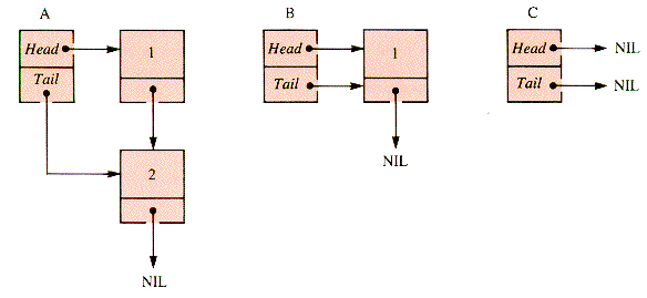
E3.3 A deletion (or insertion) procedure should be checked for performance on these lists:
Trace the action of both DeleteHead of section 3.3.4 and DeleteTail of section 3.3.4 on lists A, B, and C.
E3.4 Trace the action of the standard DeleteTail of section 3.3.4 on lists A, B, and C of E3.3 when (q
E3.5 Trace the action of the standard DeleteTail of section 3.3.4 on lists A, B, and C of E3.3 when (if q = NIL . . . ) is replaced by just the else phase. What is the result?
E3.6 Trace the action of the standard DeleteTail of section 3.3.4 on lists A, B, and C of E2.3 when the while condition is changed to: (p
E3.7 Trace the action of Copy of section 3.3.5 on lists A, B, and C of E3.3. Is it possible to change the sequence of assignments in the body of the while?
E3.8 Rewrite InsertHead of section 3.3.3 for explicit array support.
E3.9 Rewrite DeleteTail of section 3.3.4 for explicit array support.
E3.10 Rewrite Hunt of section 3.3.5 for explicit array support.
E3.11 Trace the action of IntoList of section 3.6 with insertion of values 10, 3, and - 10.
E3.12 Trace the action of LinearSort of section 3.6 on the example of section 3.6 by keeping track of all pointer variables during placement of the first and last node.
E3.13 For polynomials P2 and P3 of section 3.8, find: P2 + P3, P2 - P3, P2
Problems not immediate, but requiring no major extensions of the text material
P3.1 If the nodes of a list are numbered from 1 at Head to N at Tail, then there is an expected value, 1
P3.2 Continue the analysis of P3.1 with the assumption that x tends to be found near the head of the list. In particular, assume that finding x at nodek is twice as likely as finding it at nodek+1 for 1
P3.3 Diagram the behavior of the alteration of Copy of section 3.3.5 shown below, for the lists A, B, and C of E3.3.
P3.4 Diagram the behavior of the altered Copy of P3.3 for the lists A, B, and C of E3.3 if the while condition is changed to: (p
P3.5 Write a procedure InputSort, which inputs a stream of values, encases them in nodes, and inserts them with IntoList of section 3.6 as they are entered into an ordered list. See PG3.2.
P3.6 Determine the timing function for LinearSort of section 3.6.
P3.7 Rewrite LinearSort of section 3.6 so that the while condition is: (Spot
P3.8 Rewrite SelectionSort of section 1.4.1 to sort a linked list, using pointer variables, and determine its timing function. See PG3.3.
P3.9 Rewrite BubbleSort of section 1.4.2 to sort a linked list, using pointer variables, and determine its timing function. See PG3.4.
P3.10 Write a procedure that multiplies two linked-list polynomials.
Programs for trying it out yourself
PG3.1 Write and run program JoinUp of section 3.4.
PG3.2 Turn the procedure InputSort of P3.5 into a program that inputs a stream of values and sorts them by insertion into a linked list, then displays the values in order.
PG3.3 Turn the procedure of P3.8 into a program that inputs a stream of values, places them in a linked list, sorts them by exchange, and displays the values in order.
PG3.4 Turn P3.9 into a program that inputs a stream of values, places them into a linked list, sorts them as BubbleSort of section 1.4.2 does, and displays the values in order.
PG3.5 Write a program to accept two polynomials (supplied as coefficient-exponent pairs) and display their product.
Projects for fun; for serious students
PJ3.1 Rewrite PJ2. 1, using linked lists to track available space and in-lot cars. (The lot may be enlarged, although checking the "lot-full" test then becomes a bore.)
PJ3.2 Write a program that will manage a collection of linked-list polynomials and perform arithmetic on them as requested. The operations to be provided are addition, subtraction, multiplication, and division.
Activation
Viability
Attachment
Assignment
Partitioning
Retrieval
3.2 Linked Lists
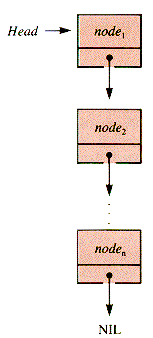
Figure 3.1
 (p-Target) is used as the name of the node pointed to by the pointer p. The value of p itself is the memory address of p
  .
. . Value is an error that will crash a program in most systems.
Figure 3.2
 Nodule, then NEW (p) has the effect shown in Figure 3.3 without an assumed initialization of p
  .
.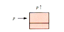
Figure 3.3
 to available space. In small programs for small applications, DISPOSE may not be needed. It will not be explicitly indicated in all the in-text algorithms where it might be useful for some applications.
3.3 Common List Operations
aList
 NIL
NIL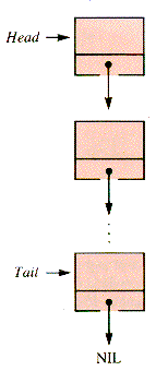
Figure 3.4

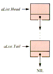
Figure 3.5
with aList do
.
.
.
endwith
3.3.1 The Empty List
{NIL-end list} {sentinel list}function Empty(aList) {O(1)} function Empty(aList)if Head = NIL if Head = u
then return TRUE then return TRUE
else return FALSE else return FALSE
endif endif
end {Empty end {Empty3.3.2 List Traversal
procedure DisplayList(aList) {O(number of nodes)p
 Head
Headwhile p
 NIL do
NodeOut(p)
p
 p
p  .Link
.Linkendwhile
end {DisplayListLT
procedure LT(aList)
PROCESS0
while CONDITION do
PROCESS1
p
 p
p  .Link
.Linkendwhile
PROCESS2
end {LTCONDITION : p
 NIL
NILPROCESS0 : p
 Head
HeadPROCESS1 : NodeOut(p)
PROCESS2 : NULL
CONDITION: p
 .Link
.Link  NIL
NILCONDITION: p
 u
uCONDITION: p
 .Link
.Link  u
uCONDITION: p
 Tail
TailCONDITION: p
 .Link
.Link  Tail
TailT(n) = t0 + n
 t1 + t2,
 .Value
  x . The two natural places to insert into a list like aList are at the head and at the tail as shown in Figure 3.6. These operations are created by changing links one at a time, in a sequence that will not destroy necessary information:
procedure InsertHead(aList,p) {O(1)if Empty(aList) then Tail
 p endif
p
 .Link
.Link  Head
HeadHead
 p
pend {InsertHead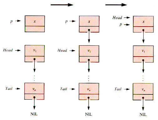
3.3.3 Insertion
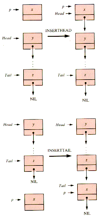
Figure 3.6
procedure InsertTail(aList,p) {O(1)if Empty(aList)
then Head
 p
pTail
 p
pendif
Tail
 .Link
.Link  p
pp
 .Link
.Link  NIL
NILTail
 p
pend {InsertTail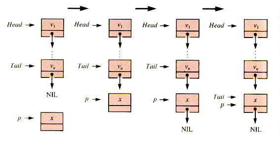
3.3.4 Deletion
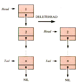
Figure 3.7
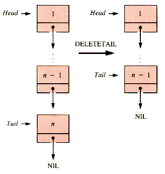
Figure 3.8
procedure DeleteHead(aList) {O(1)if Empty(aList)
then {deal with this errorelse p
 Head
HeadHead
 Head
Head  .Link
.LinkDISPOSE(p)
endif
end {DeleteHeadelse Head
 Head
Head  .Link
.Link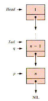
Figure 3.9
q
 .Link
.Link  p
p  .Link {since p
  .Link may be u
Tail
 q
qDISPOSE(p)
procedure DeleteTail(aList) {O(LT)if Empty(Head)
then {deal with this errorelse if Head = Tail
then Head
 Tail
Tail  .Link
.LinkDISPOSE (Tail)
else LT
endif
endif
end {DeleteTailCONDITION : p
 Tail
TailPROCESS0 : q
 Head
Headp
 q
q  .Link
.LinkPROCESS1 : q
 p
pPROCESS2 : q
 .Link
.Link  Tail
Tail  .Link
.LinkDISPOSE(Tail)
Tail
 q
qprocedure DeleteTail(Head,Tail) {O(n)if Empty(Head)
then {deal with this errorelse if Head = Tail
then Head
 Tail
Tail  .Link
.LinkDISPOSE(Tail)
else q
 Head
Headp
 q
q  .Link
.Linkwhile p
 Tail do
q
 p
pp
 p
p  .Link
.Linkendwhile
q
 .Link
.Link  Tail
Tail  .Link
.LinkDISPOSE(Tail)
Tail
 q
qendif
endif
end {DeleteTail .Link may be either NIL or u. Some possibilities for DeleteTail follow.
return
endif
q
 Head {PROCESS0
p
 q
q  .Link {PROCESS0
if p = NIL {PROCESS0then DISPOSE(q)
Head
 NIL
NILreturn
endif
while p
 .Link
.Link  NIL do {CONDITION
q
 p {PROCESS1
p
 p
p  .Link
.Linkendwhile
q
 .Link
.Link  p
p  .Link {PROCESS2
DISPOSE(p) {PROCESS2Tail
 q {PROCESS2
 .Link" when p = NIL.
procedure DeleteTail(aList) {standard DeleteTailif Empty(aList) {O(n)then {deal with this errorelse p
 Head
Headq
 p
p  .Link {q will be and stay NIL iff aList is a singleton
while p
 .Link
.Link  NIL do
q
 p
pp
 p
p  .Link
.Linkendwhile
if q = NIL
then Head
 NIL
NILelse q
 .Link
.Link  p
p  .Link
.LinkTail
 q
qendif
DISPOSE(p)
endif
end {DeleteTailprocedure DeleleTail(Head) {O(n)q
 Head {PROCESS0
p
 Head
Head  .Link {PROCESS0
while p
 .Link
.Link  u do {CONDITION
q
 p {PROCESS1
p
 p
p  .Link
.Linkendwhile
if p
 u {PROCESS2
then DISPOSE(p) .
q
 .Link
.Link  u .
u .else Head
 u .
u .if q
 u then DISPOSE (q) endif
endif {PROCESS2end {DeleteTail3.3.5 Search and Copy
function Hunt(aList,x) {O(n)p
 Head {PROCESS0
while p
 NIL do {CONDITION
if p
 .Value = x {PROCESS1
then return p endif
p
 p
p  .Link
.Linkendwhile
return NIL {PROCESS2end {Huntfunction Copy(aList)
NEW(bList) {O(n)if Empty(aList) {creates a list header, not a list value node.then bList.Head
 NIL {this is not equivalent to: {return aList.
bList.Tail
 NIL
NILreturn bList
endif
NEW(r)
bList.Head
 r
rp
 aList.Head
while p
 NIL do
q
 r
rq

 p
p 
NEW(r) {create one node aheadq
 .Link
.Link  r
rp
 p
p  .Link
.Linkendwhile
q
 Link
Link  NIL
NILbList.Tail
 q
qDISPOSE(r)
return bList
end {Copy3.4 The Upper Crust at Ballyhoo U (optional)
"IN" : Add my entry to the IN list.
"WANTIN" : Add my entry to the WANTIN list.
"SCRATCH" : Remove my entry from the IN list, or if it
is not there, from the WANTIN list.
"INLIST" : Display the entries of the IN list.
"WANTLIST" : Display the entries of the WANTIN list.
"QUIT" : Thanks, but I must go now.
program JoinUp
Write {instructions to the user.repeat
Read(Command)
case of Command
"IN": if InCount < 25
then me
 WhoAreYou
InsertTail(IN,me)
InCount
 InCount + 1
else Write {explanationme
 WhoAreYou
InsertTail(WANTIN,me)
endif
"WANTIN": me
 WhoAreYou
InsertTail(WANTIN,me)
"SCRATCH": me
 WhoAreYou
p
 Hunt(IN,me)
if p
 NIL
NILthen Scratch(IN,p)
else p
 Hunt(WANTIN,me)
if p
 NIL
NILthen Scratch(WANTIN,p)
else {report failure to find meendif
endif
"INLIST" : ListOut(IN)
"WANTLIST" : ListOut(WANTIN)
"QUIT" : exit
else: {Provide the user with a list{of legitimate commands.endcase
forever
end {JoinUp .Link, instead of p:
procedure Scratch(aList,p) {O(n)if p = Head
then DeleteHead(aList)
else q
 Head
Headwhile q
 .Link
.Link  p do
p doq
 q
q  .Link
.Linkendwhile
q
 .Link
.Link  p
p  .Link
.LinkDISPOSE(p)
endif
end {Scratchprogram Floodgate {O(n)m
 25 - InCount
for i = 1 to m do
NEW(p)
p

 WANTIN.Head
DeleteHead(WANTIN)
InsertTail(IN,p)
InCount
 InCount + 1
next i
end {Floodgate3.5 Array Support for Linked Lists
Head
 Link[0]
p
 i
ip
 .Value
  Value[i]
p
 .Link
.Link  Link[i]
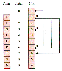
Figure 3.10
ALT
procedure ALT(Value,Link) {0(n)Next
 Link[0] {PROCESS0
while Next
 0 do {CONDITION
PROCESS1(Next)
Next
 Link[Next]
endwhile
PROCESS2
end {ALTValue[10]
 "-"
"-"Link[10]
 Link[7]
Link[7]
 10
10PROCESS0: Length
 0
0Next
 Link[0]
PROCESS1: Length
 Length + 1
procedure DeleteHead {O(1)if Link[0] = 0
then {deal with this errorelse Link[0]
 Link[Link[0]]
endif
end {DeleteHead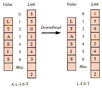
Figure 3.11
procedure InsertTail(k) {O(1)if Link[0] = 0
then Link[0]
 k
kendif
Link[Link[Max + 1]]
 k
kLink[Max + 1]
 k
kLink[k]
 0
0end {InsertTail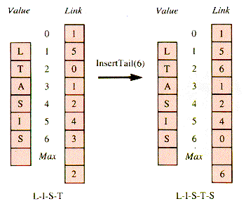
Figure 3.12
GetSpace(k)
InsertTail(k)
 Max, and the space occupied by deleted values is just ignored.
3.6 Ordered Lists
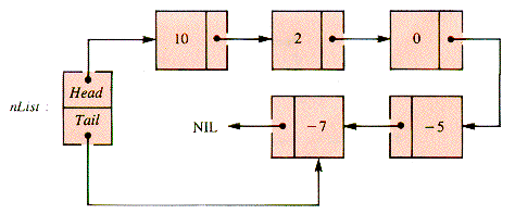
Figure 3.13
NumNode = RECORD
Value: INTEGER
Link :
 NumNode
END {NumNode{determine xNEW(xNode)
xNode
 .Value
  x
x NIL, the entire list is available to define an insertion position.
CONDITION : p
 .Link
.Link  Spot
SpotPROCESS0 : p
 Head
HeadPROCESS1 : Next
 p
p  .Link
.Linkif x
 Next
Next  .Value then exit endif
PROCESS2 : xNode
 .Link
.Link  p
p  .Link
.Linkp
 .Link
.Link  xNode
xNodeprocedure IntoList(nList,xNode,Spot) {O(n)if Empty(nList)
then Head
 xNode
xNodeTail
 xNode
xNodexNode
 .Link
.Link  NIL
NILreturn
endif
x
 xNode
xNode  .Value
if (x
 Head
Head  .Value) OR (Spot = Head)
then xNode
 .Link
.Link  Head {new Head node
Head
 xNode
xNodeelse p
 Head {LT
while p
 .Link
.Link  Spot do
Next
 p
p  .Link
.Linkif x
 Next
Next  .Value then exit endif
p
 p
p  .Link
.Linkendwhile
xNode
 .Link
.Link  p
p  .Link
.Linkp
 .Link
.Link  xNode
xNodeendif
end {IntoList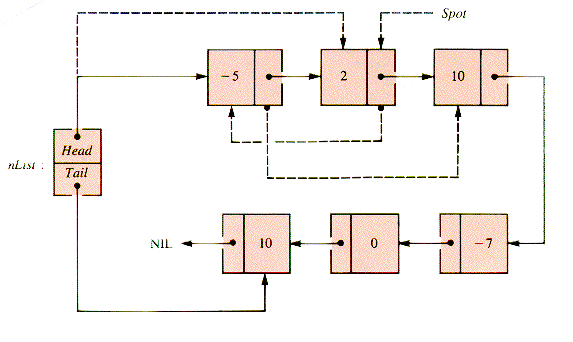
Figure 3.14
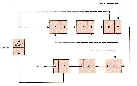
Figure 3.15
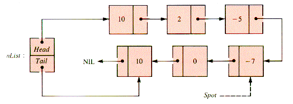
Figure 3.16
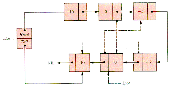
Figure 3.17
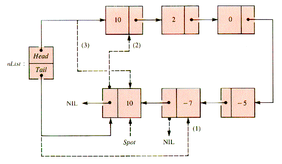
Figure 3.18
 .Link) after Spot is excised from the list. Hence the sorting procedure becomes:
procedure LinearSort(nList) {O(n2)if Empty(nList)
then {deal with this errorelse Spot
 Head
Head  .Link
.Linkif Spot = NIL then return endif
Prior
 Head
Headwhile Spot
 .Link
.Link  NIL do
SpotLink
 Spot
Spot  .Link
.LinkPrior
 .Link
.Link  SpotLink
IntoList(nList,Spot,SpotLink)
if Prior
 .Link
.Link  SpotLink
then Prior
 Spot
Spotendif
Spot
 SpotLink
endwhile
Prior
 .Link
.Link  NIL
NILIntoList(nList,Spot,NIL)
if Tail
 .Link
.Link  NIL
NILthen Tail
 Prior
Priorendif
endif
end {LinearSort3.7 Circular Lists
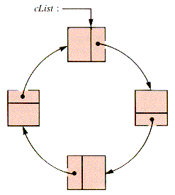
Figure 3.19
3.8 Polynomial Arithmetic (optional)
P1: 31x17 - x11 + 5x4 + 10x3 - 3
P2: 7x17 + 4x6 - 2x2 + 8
P3: x11- 5x4 + x2 + 3
 P1 + P3 changes the number of CE pairs needed to describe P1.
PolyNode = RECORD
exp : INTEGER
Coef : REAL
Link :
 PolyNode
END {PolyNode
Figure 3.20
function PolyAdd(P,Q)
PAQ
 u
uwhile P
 u AND Q
  u do
u doNEW(R)
case
P
 .exp > Q
  .exp : R
 P
P
P
 P
P  .Link
.LinkInsertTail (PAQ,R)
P
 .exp = Q
  .exp : R
  .exp
.exp  P
P  .exp
.expR
 .Coef
.Coef  P
P  .Coef + Q
  .Coef
.CoefP
 P
P  .Link
.LinkQ
 Q
Q  .Link
.Linkif R
 .Coef
.Coef  O
Othen InsertTail(PAQ,R)
endif
P
 .exp < Q
  .exp : R
 Q
Q 
Q
 Q
Q  .Link
.LinkInsertTail(PAQ,R)
endcase
endwhile
if P = u
then Rest
 Q
Qelse Rest
 P
Pendif
while Rest
 u do
u doNEW(R)
R

 Rest
Rest
InsertTail(PAQ ,R)
Rest
 Rest
Rest  .Link
.Linkendwhile
return PAQ
end {PolyAdd3.9 Arithmetic of Unbounded Precision (optional)
$197,800,400,650.23
 1011 would be an adequate representation of the number above.
743.1 = 7
 102 + 4
  101 + 3
  100 + 1
  10-1
10-1
Figure 3.21
Summary
Exercises
 p
p .Link) is omitted. What is the result?
 NIL). What is the result?
 P3, and both the quotient Q and remainder R of P2 / P3.
Problems
 ex
ex  N for the number of the node located by Hunt of section 3.3.5. Assume that every node is equally likely to contain the searched-for value x and that there is only a 50 percent chance that x is a node value at all. Determine T(N) for Hunt, as a function of ex.
 k
k  N - 1. In effect, find ex.
NEW(q)
bList. Head
 q
qp
 aList.Head
while p
 NIL do
q

 p
p 
NEW(r)
q
 .Link
.Link  r
rq
 r
rp
 p
p  .Link
.Linkendwhile
q
 .Link
.Link  NIL
NILreturn bList
.
.
.
 .Link
.Link  NIL).
NIL). NIL).
NIL).Programs
Projects


