Dear Ann Landers:
Why is it that whenever I lose anything, it is always
in the last place I look?
--Dizzy Lizzy
Dear Liz:
Because when you find it you stop looking--and
that's the last place you looked.
Although searching and sorting may appear mundane, the speed with which they can be carried out largely determines whether a particular application of the computer is practical (and "cost-effective'") or not. Estimates indicate that about one-fourth of the processing time in computer centers is spent just sorting. The relation between sorting and searching will become apparent in this chapter. If one can be done faster, so can the other. The choice of data structures is always important in algorithm design and is the key to the evolution of good (that is, efficient) searching and sorting procedures. The basic data structures studied in the preceding chapters (arrays, lists, and binary trees) are used in the design of efficient procedures.
Normally, the objects stored, searched for, and sorted are records. In sorting, one field of the records, called the sort key, is chosen as the basis for the sort. Thus, in a payroll application, an employee name field might be the key for an alphabetical ordering, while a salary field might serve as the basis for a sort to determine an ordering by amount of earnings. At times the sort key can be a combination of fields. As an example, we may desire to sort with name as the primary key and zip code as the secondary key. For simplicity it will be assumed in this chapter that the objects being sorted are integer numbers. However, any variable type could have been assumed. For sorting purposes, the only requirement is that, given any two objects, it is possible to tell which precedes the other.
Searching normally involves comparing records to a given search key value. The goal is to determine whether there exists among the records of the data base a record with key equal to that of the search key. If the key value can be matched, then a pointer to the record with the matching value must be returned. The basic principle for shortening search times is to organize the data base so that the search can be focused quickly on the part of the data base that will contain the desired record, if it is present.
The chapter first explores simple linear, binary, and interpolation searches and a number of elementary sorting algorithms, such as the bubble sort and the insertion sort. These lead to more advanced methods for sorting based on a special binary tree called a heap. Next, an application of recursion yields another fast sort, quicksort.
Some of the algorithms developed in the text are fairly complex and difficult, if not impossible, to analyze mathematically. For this reason the last topic considered in the chapter is the use of simulation as a tool in discovering the behavior and efficiency of such complex algorithms.
The chapter concludes with a summary of the strengths and weaknesses of each approach introduced. Knuth [1973b] and Wirth [1976] discuss many searching and sorting algorithms that are not dealt with in this text. Knuth also contains mathematical analyses of many of these algorithms.
Three simple searches are applicable when records are stored in arrays: (1) linear search, (2) binary search, and (3) interpolation search. You probably have all used these methods in everyday activities. Understanding their limitations and how they work will help you see the need for the more complex structures and algorithms of later sections.
A linear search is so named because it proceeds in sequence, linearly through an array. Suppose data in Figure 8.1 is an array of integers.* The task is to determine whether the number stored in the variable key is in the array, and if so, what its index is.
* To simplify the explanation in this chapter, the 0th array position will be ignored, and data stored in arrays will start in position 1 unless otherwise noted.
One obvious method would be to traverse the data array, checking each element of data to see if it contains the same value as key. If an element currently being processed did contain the same value as key, its index would simply be returned, and the search would be complete. Arriving at the end of data without having found the key value would mean that no element with that value is stored in the array. This procedure is easily implemented using a loop structure (as in the following function). The worst-case time required for its execution will be of the order n, written O(n), where n is the length of the data array. In particular, if the value being sought is in element i of the array, it will take O(i) time to find it. The linear search is implemented as follows:
A special but common case is when the search is always for a key known to be stored in the array, and each key stored is distinct and equally likely to be the search key. This is like standing in front of a locked door with a bunch of keys. You need to find the key that opens the door from among n keys in arbitrary order on your key-ring. The average time for such a search would be O(n/2). That is, on the average, you would look at half the keys, or half the elements of the array, before finding the right one.
Thus the procedure called linear search is so named, not only because it proceeds linearly through an array, but also because its processing time increases linearly with n; when n is doubled, the time required to complete the search is doubled.
Occasionally programming tricks can be used to enhance efficiency. In this case paying attention to some details produces a trick that can pay off by saving processing time. The straightforward implementation of the linear search requires a test (loc
Place the search key in element n + 1 of data. Then, in implementing the linear search, there is no need to test for the end of the array before checking the next element. Since the array is now considered to be (n + 1) elements in length, we are certain to find the search key before we "fall off the end." After the loop is exited, note the element in which key was found, and test to see if it was the (n + 1)th element, which means that the search was unsuccessful. Thus only one test (data[loc].key ! = key) must be performed. This saves n tests in unsuccessful searches, and i tests in successful searches, when the search key appears in element i of data. This simple modification of the basic linear search can easily produce significant time savings (20 to 50 percent). In general, whenever loops are modified to reduce the tests or processing they perform, execution time is saved each time through the loop. The more efficient linear search implementation appears as follows:
Another way to save time in a linear search is to order the records in the array. One way to do this is to store them in decreasing order of key value. The linear search can then be modified by terminating the search as soon as a record is reached whose key value is less than the search key. The desired record cannot be in the array past that point. Although this results in extra comparisons for successful searches, time is saved overall when unsuccessful searches occur frequently enough.
It is also possible, if the frequency with which records will be retrieved is known, to store the records in decreasing order of retrieval frequency. The most frequently retrieved record will then be at the top of the array. This approach significantly improves search efficiency when the desired record is likely to be near the top of the array. In fact, if the frequencies decrease rapidly enough, the average search time for the linear search will be a small constant.
Certainly no one does a linear search to look for a phone number in the telephone directory. Imagine trying to do so in the directory for New York City or any other large city! But there are ways to carry out the search so that the name is found in a few seconds, even from among a few million names. The structure of the telephone directory is the clue to the solution, which takes advantage of the alphabetical ordering of the entries in the phone book.
Assume that the numbers stored in data are arranged in decreasing order, as in Figure 8.2. They are said to be sorted in decreasing order. Since a telephone book is sorted in alphabetical order, one of the things most people do by habit when using the telephone directory is to flip the directory open toward the front, middle, or back depending on the location in the alphabet of the name being sought. If the page opened to has names farther down in the alphabet, the search name cannot be on that page or anywhere in the directory to its right. It can only be to the left of the selected page. This process of elimination is behind the search technique called binary search. It is not difficult to see why this search technique is called binary. Every time a test is made in the search, there are two choices. In the telephone book example, search either half of the remaining pages for the name.
A binary search is also a good strategy for winning the game of twenty questions, which requires guessing the identity of an object after finding out if it is in the animal, the mineral, or the vegetable category. Twenty question with "yes" or "no" answers are allowed. Selecting each question so that about half the remaining possibilities are eliminated, no matter what the answer, is best. (For example, given the animal category, "Is the object male or female"?) In this way 220, or over a million, objects can be distinguished.
In twenty questions it is difficult to select a question that makes close to a 50-50 split of the remaining possibilities. However, if you are asked to determine a number known to lie between 1 and 1024 by asking yes-no questions, it is easy to do so. Ask, "Is it greater than 512?" and continue splitting the remaining possibilities in half. No more than 10 such questions are needed to find the number from among the 210 (1024) initial possibilities. Similarly, when searching for a specific key value among 2n records, at most n key comparisons are needed to determine whether it is present, as long as each comparison splits the remaining collection of records into two parts that differ in size by at most one.
When searching data stored in arbitrary order in an array, there is no reason to expect the search key to be in any particular region of the array. However, when the data have been stored in sorted order, the situation is different. It is possible to check the middle element to see if the search key is there. If it is, the program would note its location and terminate the search. If the key is not there, then if the search key is greater than the key in the middle element, eliminate the middle element and all elements below it from consideration. If the desired record is in data at all, it must be above the middle element. Similarly, if the search key is less than the key in the middle element, eliminate the middle element and all elements above it. In any event, at most half the elements remain to be considered, and the same procedure can then be applied to the appropriate half: either elements 1 to [mid-1] or elements [mid+1] to n. Mid is a variable that points to the middle element.
For example, if mid is 10, then the search key value, 25, is not greater than data[mid], 78. Hence, if it is in data at all, it must be between positions mid+1 and n--11 and 20. Taking 15 as the middle element of these, the new mid value is 15. Key is less than data [mid], 32. Hence we need to search between mid+1 and 20-16 and 20. With a new mid value of 18, key is greater than data [mid], 13. Now search only between 16 and 17. The next mid value is 16, and the key is found.
The basic structure of the binary search algorithm is a loop, as shown in the following function.
Mid is initialized to the middle element of data, top to 1, and bottom to n. Top and bottom are variables that point to the top and bottom elements of the consecutive elements left to be searched, all others having been eliminated from consideration. In the loop body, test for key equal to data [mid]. If the equality is true, the program exits the loop and the search is done, since key has been found at element mid. If not, top and bottom must be updated to reflect the new sequence of elements that are to be searched. This updating must set bottom to mid whenever key is greater than data [mid], and top to mid + 1 otherwise. The test for continuing the loop involves checking whether key was found, and whether any elements are left to be searched between top and bottom. The search is terminated as soon as the desired entry is found or as soon as it is concluded that the entry is not present. Loc will be zero if the key value was not found and will index its location in data if found.
How much time is required by the binary search algorithm in the worst case? Each pass through the loop requires at most a constant amount of work. The time to execute the algorithm will then be determined by the number of passes through the loop, plus, of course, a constant time for initialization and finalization. What is the greatest number of loop iterations executed?
In each pass through the loop, the search involves at most half the elements that were under consideration during the preceding pass through the loop. Starting with n elements, after one pass through the loop at most 1/2n elements are left, after two passes through the loop at most 1/2(1/2)n elements, after three passes at most 1/2(1/2)2n elements, and after k passes at most 1/2(1/2)k-1n or 1/2kn elements. This number, 1/2kn, is less than 1 when -k + 1g n < 0 or when k > 1g n. This means that the loop cannot be executed more than
Sometimes, telephone directories, like dictionaries and encyclopedias, have tabs so that users can flip open the book to the beginning of the section containing entries with a specific first letter and gauge whether to search toward the front, middle, or back pages of the section. The tabs have been inserted or interpolated within the data to guide the search. This represents a generalization of the binary search called the interpolation search. The topic will not be pursued in detail, but note that this technique allows the elimination of greater fractions of the remaining names than does a binary search. Not surprisingly, this tends to reduce the execution time.
When n is large, the binary search takes much less time, in the worst case, than the linear search. This is because it makes 1g n rather than n comparisons, going through its loop body 1g n rather than n times. However, the steps performed in the loop body of the binary search are more complex and more time-consuming than the steps performed in the loop body for the linear search. Hence it is possible, for smaller values of n, that the linear search will be faster. Similarly, the interpolation search will need to perform more complex steps in its loop body, even though it may need to loop fewer times than the binary search.
Of course the binary and extrapolation searches require sorted data. When only a few searches are to be made or when n is small, it may not pay to spend time to sort the data first. For repeated searching or large n, the efficiencies of the binary and extrapolation searches easily overcome the cost of sorting.
We now turn our attention to three simple sorting methods applicable to records stored in arrays: (1) maximum entry sort, (2) bubble sort, and (3) insertion sort. They are also applicable to records stored in lists. Understanding their limitations and how they work sets the stage for the more complex structures and algorithms of the next section.
Perhaps the most straightforward way to sort numbers in an array into decreasing* order is to begin by placing the largest number in element 1. The next largest number is then placed into element 2, and so on. The maximum entry sort repeatedly finds the next largest array entry and places it in its proper position in the array. Suppose the point has been reached in this procedure where the k largest numbers have been properly placed into the first k elements of the array data. Assume a variable next points to the element of data into which the next largest element is to be placed. Next must now be updated to next + 1 so that it contains the value k + 1, as indicated in Figure 8.3.
* The sorting programs assume that decreasing order is desired. They can easily be modified to sort in increasing order.
Assume that a function maxloc exists, with parameters data, next, and n, the array length. Maxloc returns with its value indexing the largest element between the nextth and the nth elements of data. The sort may then be obtained by a loop in which maxloc is invoked (n - 1 times, with next taking on values 1, 2, . . . , n - 1, respectively, on each call. Within the loop, when each call to maxloc is made, an exchange between data [next] and data[maxloc] occurs.
Maxloc might be implemented by traversing the elements next to n of data. Each time a new element is accessed, it is compared to a variable, largest, containing the largest entry seen so far in this traversal. If the new element is greater than largest, largest is set to the new element value, and maxloc is set to point to the location of the new element in data.
This algorithm is probably similar to what most peole do instinctively when confronted with a small sorting problem. It may be implemented as in the procedure maxentrysort.
For the simple record used here for illustration, the interchange function is as follows.
How much time does this implementation of the maximum entry sort take? One interchange is made on each call to maxloc for a total of n - 1 interchanges. The number of comparisons is (n - k) on the call to maxloc, when next has the value k. The total number of comparisons is (n - 1) + (n - 2) + . . . + 2 + 1, which sums to [n(n - 1)]/2. Thus the time is determined by the time of the (n - 1) interchanges plus the time of the [n(n - 1)]/2 comparisons. Each interchange takes a constant amount of time, and each comparison takes, at most, a constant amount of time. The result is O(n2) time. This means that if n is doubled or tripled, the time will increase by a factor of about 22, or 4, and 32, or 9, respectively, when n is large. For n = 105, the time is roughly proportional to 1/2 1010, which is within a factor of 100 of 1013, the guide for feasibility presented in Chapter 1. Quicker algorithms are obviously needed for large n, and even perhaps for small n. The next elementary sort technique offers some improvement.
The bubble sort gets its name from the way smaller entries "sink" to the bottom of the array during the sort while larger entries "bubble up" to the top. To carry out the bubble sort on the array shown in Figure 8.4(a), traverse the array, comparing two adjacent elements, starting with the first two, and ending with the last two. If the [i + 1]th element value exceeds the ith, interchange the two element values.When a traversal is completed, it is called a pass through the array. Continue making passes until a pass occurs in which no interchanges are required.
In the example, after pass 1, the array looks like Figure 8.4(b). Since at least one interchange was made, another pass is made, yielding Figure 8.4(c). Again, at least one interchange was made, so the program must make another pass.
Will this process continue forever making passes, or eventually stop? Clearly, once it stops since no interchanges were made on the last pass, the array is sorted. If any number were out of order, at least one interchange would have been made during that pass.
Notice that after the first pass the smallest entry, 3, was at the bottom of the array. After the second pass the two smallest entries, 10 and 3, were in order at the bottom of the array. This was not accidental. Notice that the two smallest entries will never be moved, and the third smallest element (13 in this case) will be encountered on the next pass. Once it is encountered, it will always be interchanged with the adjacent lower record to which it is compared. It will eventually come to rest just above the second smallest entry.
In general, after the kth pass, the k smallest entries will be in order in the bottom k elements of the array. Of course, more than the k smallest may be in order at this point, but only k can be guaranteed. Hence the array will be in sorted order after at most n - 1 passes. The procedure can therefore be modified to compare down to only the [n - k]th element on the kth pass. The bubble sort is implemented with the following function.
If the array were initially given in sorted order, only one pass would be required, and the time would be proportional to n. If the array were initially given in reverse sorted order, then n - 1 passes would be required, with (n - 1 - k) interchanges and comparisons. This is the worst case, and takes time determined by the
The next sort to be considered is insertion sort. An insertion sort works by assuming that all entries in the array are already in sorted order and inserting the next entry in its proper place in the order. Figure 8.5 presents an example of an insertion sort.
In this example the same array, data, is used as for the bubble sort. Each record is processed in turn, starting from the second. Figure 8.5(a) represents the situation after processing of the first six records. The seventh is yet to be processed. It is processed, as are all the other records, by assuming the preceding records are already in sorted order. Notice that records 1-6 are in order. To insert the seventh record, 75, into its proper place among the first seven records, compare record 7 with its predecessor, record 6. Since 75 exceeds 10, it should go somewhere higher up in the array, so compare it to the predecessor of record 6, record 5. Since 75 exceeds 32, compare it to the predecessor of record 5, record 4.
Again, 75 exceeds that element's value of 32, so compare it to its predecessor's value, 65. The last comparison is with 78. Since 75 does not exceed 78, record 7 must be inserted between record 2, where 78 is now, and record 3. To do this, move records 3 to 6 down one element, respectively, and place 75 in record 3. The result is Figure 8.5(b).
K has been updated by 1, so it points to the next record to be inserted. This algorithm for an insertion sort can be described by a loop structure in which k varies from 2 to n, as in the following function.
Within the loop, process the kth record by inserting it properly among the top k elements. This may be accomplished by another loop, in which record k is compared to each consecutive predecessor until it does not exceed the current predecessor record. It is inserted at that point in the array. As an exercise, you should modify the insertionsort program to incorporate the programming trick of Section 8.2.2. In Table 8.1 (see Section 8.7), this is referred to as the modified insertion sort.
If the initial array were given in sorted order, the insertion of the kth record would require one comparison and no insertions. The total time would be O(n - 1). If the initial array were given in reverse sorted order, the insertion of the kth record would require (k - 1) comparisons, and the kth record would have to be inserted at the top of the array. To accomplish this, each of the (k - 1) records must be moved down one element. The total time will be the time for the 1 + 2 +
In the three implementations for the sorting algorithms, it was assumed that the interchanges taking place were actually interchanges of records. When records are large, it takes appreciably more time to move a record than it does to move a single pointer to the record. Consequently significant amounts of time can be saved by keeping an array, p, of indexes or pointers to the records. The entries of this array can then be kept in order, so that p[i] indexes or points to the ith record in sorted order. Interchanging indexes or pointers takes less time than for records but uses more memory (which is an added expense). This is another example of trading time for storage. In the procedures shown for maximum entry sort, bubble sort, and insertion sort, the interchange operations would then apply to the array p, and the comparison operations would apply to the actual records indexed or pointed to by i.
The next question is, can we improve the insertion sort? We could try to improve it by changing how the search is done for the correct location of the kth entry. In effect, the insertion sort traversed linearly through records [k - 1] to 1 to insert the kth record. Instead, we could do a binary search of the consecutive elements 1 to [k - 1]. We will then know where to insert the kth record. This will reduce the 1 + 2 +
What else can be tried to improve the insertion sort? Aha, lists! Recall that lists are convenient for insertions, so simply represent the records in a list rather than an array. Then, once you know where to insert a record, merely change two pointers. Thus the 1 + 2 +
Wait! We are not yet defeated in our quest for a faster insertion sort. Use a pointer array, assuming enough storage is available, to tell where all the records are on the list. This allows selection of the list records as in Chapter 2. The situation is then as shown in Figure 8.6.
Numberlist is the head of the list of records in the illustration. Suppose the first six records have been properly processed as in the insertion sort, and the seventh is to be processed next. A binary search can now be done, since the middle record, among 1 to 6, will be indexed by the middle entry of elements 1 to 6 of the pointer array. Thus it is possible, in 1g 6 time, to determine where the seventh record is to be inserted. The insertion will require the changing of two pointers. But here's the rub! To maintain the pointer array, it must have its seventh element inserted in the corresponding position of the pointer array. We have merely succeeded in transferring the insertion problem to the pointer array; we have not eliminated it!
Although these attempts to find a faster sorting algorithm have so far not been successful, they provide insight into the binary search and sorting problems. First, notice that except for the binary search, all the searching and sorting algorithms so far considered may be applied to records stored in lists as well as in arrays. Observe that to achieve both a search in binary search time (lg n) and fast insertions and deletions, a linked type structure is needed, as well as some way to eliminate from consideration a significant fraction of the records. A second observation is that the original insertion sort would be faster if the length of the array in which each insertion is made were shorter. We must somehow break up the array of records to be sorted, so that the individual insertions do not involve all of the previous records. These observations lead to the ideas behind heapsort and quicksort, two faster sorting algorithms.
In this section and the next, two less obvious but faster sorts are considered. These two sorts, heapsort and quicksort, were developed from different points of view and as a result have different advantages.
Heapsorts use the concept of a heap. A heap is a binary tree with the property that all records stored in nodes are in sorted order along the path from each node back to the root. The tree of Figure 8.7 is not a heap. Its records are not in sorted order along the path from each node to the root. For example, the path from node 10 (where 123 is stored) to the root is not in sorted order. That path has records 123, 10, 32 and 100. (The nodes in this chapter are numbered like the nodes on trees in Chapter 7 and are referred to by their number.) Notice that the tree has the same information as the data array, but the information has been spread out along different paths.
Figure 8.8(a) is a heap storing the same information. It is one of many heaps that can be created to store the information. Since the path from every node to the root is in sorted order, the record at the root of a heap must be as great as any other in the tree. The same holds for all subtrees. The record at the root of any subtree must be at least as great as any other record in the subtree. The root record may then be taken as the first record in a sorted output of the information stored in the tree.
To sort, output 536 first, and then remove it from the tree. Now suppose that somehow the records can be rearranged in the tree to create a new heap--a process called reheaping. The result might look like Figure 8.8(b). This tree has one less node than the original. Clearly, this process of removing the root can be repeated, outputting it next in the sorted output, and reheaping. When all the records have been output in sorted order, the remaining tree will be the null binary tree (the heap will be empty), and a sort will have been obtained. The algorithm is stated simply:
To perform a heapsort:
1. Create a heap.
2. While the heap is not empty
a. output the record at the root of the heap,
b. remove it from the heap, and
c. reheap.
As stated, the algorithm is not detailed enough. It does not specify how to create a heap (step 1) or how to reheap (step 2).
Consider the heap of Figure 8.8(a) with one new record as in Figure 8.8(c). Notice that all paths are in order, except for the path from the new record at node 21 to the root. This prevents this tree from being a heap. To make it a heap, the insertion sort idea may be useful. Insert the new record at its proper place along the already sorted path from its predecessor node to the root, and allow 425 to work its way up along the path as far as it can go the reach its proper place. This can be done by comparing 425 to its predecessor and interchanging if it exceeds its predecessor's value. In this case, it does exceed that value, so interchange to obtain the tree shown in Figure 8.9(a).
All other paths remain sorted, as before. Now compare 425 at node 10 with its predecessor. Since it exceeds 123, interchange again to obtain Figure 8.9(b). Finally, compare 425 with its predecessor's value, and interchange to obtain Figure 8.9(c).
At this point, when 425 is compared to its predecessor's value, the 425 has reached its proper place. All paths must now be in order, since the path from node10 to the root is in order, and the interchanges have not disturbed the order along any other path.
This gives us the means to create a heap:
Start with records stored in the complete binary tree and process each node in turn, starting with node 2 and ending with node n.
The processing of the ith node is exactly the same processing as was done on the new record 425. Since nodes 1 to i - 1 will already have been processed prior to processing node i, the binary tree consisting of nodes 1 to i - 1 will already be a heap. Processing node i then, in effect, treats the record at node i as a new record and creates a new heap. For the example of twenty records, this procedure leads to the heap of Figure 8.8(a).
In order to analyze the time required, recall that the number of nodes n and the depth of a complete binary tree are related by
This is important. Since the heaps dealt with initially in our heapsort algorithm are complete, their depth is O(lg (n)).
We now analyze the time required to create a heap by this algorithm. Starting from a complete binary tree is important. For instance, if we started with the binary tree shown in Figure 8.10, this algorithm would be equivalent to the original insertion sort of Section 8.3.4.
The heap creation algorithm does a total amount of work determined by the sum of the number of comparisons and interchanges needed in processing each node. A node at depth k cannot require more than k comparisons and k interchanges in its processing. The worst-case time will be achieved for any initial tree in which the numbers stored at nodes 1, 2, 3, . . . , n form an increasing sequence. For instance, if the integer i is stored at node i, for i = 1, 2, . . . , n, we obtain such an increasing sequence. If n is 15, the tree will be as shown in Figure 8.11.
It can be shown that the total time for such a tree to be turned into a heap by the algorithm is proportional to
For a tree of depth d, a better procedure for creating a heap is to start at node number 2d-1 - 1, the rightmost node at depth d - 1. Even better, start at
Consider the initial complete binary tree in Figure 8.12(a). Start at node 5 ( =
The subtree with node 5 (94) as root is now a heap. Move to node 4, and the similar comparisons reveal that it is already a heap. Move to node 3, compare its successors 29 and 30, and then compare the larger to 16. Since 30 exceeds 16, interchange 30 and 16 to obtain Figure 8.12(c).
The subtree of node 3 is a heap, so move to node 2. Compare its successors 57 and 94, and then compare the larger to 14. Interchange 94 and 14 to obtain Figure 8.12(d).
At this point, notice that all nodes processed so far must be the roots of subtrees that remain heaps, except perhaps for the root of the subtree, where 14 now appears after the interchange. This subtree need not be a heap and, in fact, is not in this case. You can make it a heap by applying the same process to the node where 14 is currently stored, node 5. Compare its two successors and then compare the larger of those with 14. Then interchange 14 and 83 to obtain Figure 8.12(e).
The subtree with root node 2 is now a heap, and the processing of node 2 is complete. Notice that all nodes processed so far are roots of subtrees that are heaps. The last node to be processed is now node 1. Compare its successors, 94 and 30. Since the larger, 94, exceeds 18, interchange to obtain Figure 8.12(f).
The 18 from the node being processed, node 1, has now moved down to node 2. Hence its subtree may no longer be a heap. Apply the process to node 2. The 18 can move down again and will continue to move down until it either becomes situated at a terminal node or becomes the root of a subtree that remains a heap. In this case, it should be compared with 83, the larger of its two successors, and interchanged to get Figure 8.12(g).
At this point, you can see that 18 is the root of a heap by comparing it to the larger of its two successors. Processing of node 1 has been completed, and the heap has been created. The heap obtained from the original example with this algorithm is Figure 8.12(h). Notice that this heap differs from that in Figure 8.8(a). As mentioned earlier, more than one heap can be constructed to store the same data.
Without analyzing this heap creation algorithm in detail, the result can be stated. This procedure is actually only O(n). This heap creation algorithm is faster than that of the last section because few nodes must move down long paths. In the other algorithm, many nodes may move up long paths. A use for this linear time heap creation algorithm will be demonstrated in another context in Section 9.2, Priority Queues.
One way to implement the heap creation algorithm is to make use of a function, or routine, that works on a binary tree whose left and right subtrees are already heaps. The function does the "shifting" down of the root record until it becomes the root of a subtree that remains a heap, or until it reaches a terminal node. This "shift" routine need not do the interchanging along the way. Instead it can determine the final position of the root being shifted down, moving each record along that path to its predecessor, finally placing the root where it belongs.
Notice that the first heap creation algorithm requires testing the record being inserted along a path to the root against its current predecessor. Before this can be done, the program must test for whether or not there is a predecessor--that is, whether the record has already reached the root. This test must precede every comparison. Similarly, in the second heap creation algorithm, the record being shifted down must be tested against its successors. Before doing this, it is necessary to test whether there are successors.
These tests can be avoided by always putting "plus infinity" at the root of the initial complete binary tree for the first algorithm, and "negative infinity" at the subtrees of all terminal nodes for the second algorithm. This is similar in effect to adding the search key to the end of the array in the linear search algorithm. Plus infinity and negative infinity stand for, respectively, any number larger or smaller than the numbers appearing in the binary tree. In this way, a record being inserted along a path in the first algorithm will never reach the root (so it will always have a predecessor with which it may be compared), and a record being shifted down in the second algorithm will always have successor nodes (since it will never become a terminal node).
Think of step 1 of the heap sorting algorithm as phase I, in which a heap is created. The execution of step 2 until the records are sorted is phase II. In phase II, the root element of the heap is removed and output. The program must then reheap. This may be done in two ways.
One is to allow the "gap" created at the root by removal of its record to shift down by comparing its two successors and interchanging the larger of the two successors with the gap, then repeating this process until the gap is at a terminal node. A convenient way to do this is to replace the record removed from the root by a "negative infinity" and invoke the shift down function referred to earlier for the second algorithm.
A second way to reheap is to replace the gap with the rightmost record at greatest depth. (Actually, any record with no successors will do.) The same shift function may be invoked to reheap.
Since the length of the longest path in a complete binary tree is O(lg n), the reheaping after each record is removed can take time at most O(lg n). Because n records will ultimately be removed, the total time required for phase II will be at most O(n lg n). For either implementation of phase I, the total heapsort time is O(n lg n). This was achieved by "spreading out" the records along paths of a complete binary tree, and, in effect, doing insertions only along the path from a record to the root.
We have been dealing with a max heap, in which the largest record is at the top. A min heap, with the smallest record at the top, is dealt with similarly. The only difference is that interchanging occurs when a successor's key is smaller, rather than larger.
A detailed version of the heapsort algorithm can now be developed. You have now seen a number of ways to create a heap and to reheap. We will use the second heap creation algorithm for phase I and the second reheaping algorithm for phase II. Both algorithms use the shift function.
To proceed we must decide on an implementation of the binary tree data structure. The binary tree used in heapsort is initially complete. The required processing involves predecessors and successors of nodes. Sequential representation for the binary tree is ideal, so we use it. The binary tree is stored in the data array and consists of n records.
Storage is needed for the sorted version of data. Although another array may seem necessary for this purpose, we will use only the data array. The algorithm, after creating a heap (in data), continually takes the root record as the next record in the sorted output and then reheaps. Before reheaping, the rightmost record at the lowest level of the heap is placed at the root. The storage vacated by that rightmost record will no longer be needed. We choose to store the output record there. You should convince yourself that this will result in the records appearing in data in reverse sorted order upon termination. To remedy this, we write shift so that it produces min heaps. The records will then appear in correct sorted order upon termination.
Shift has parameters data, root, and last. Root points to the root of a subtree, and last points to the node of the original heap that is currently the rightmost node at greatest depth. The nodes last+1 to n are currently storing the already sorted n-last output records. Whenever shift is invoked, the left and right subtrees of root (excluding nodes last+1 to n) are assumed to be heaps. Shift returns after reheaping, by allowing the root record to move down to its final position. This is done by first storing the key value and record of the initial root record in keyvalue and recordvalue, respectively. Ptr points to the node currently being considered as the final position for the initial root record. This will be the final position if either of the following two conditions is met.
1. The successor record of ptr with minimum key value has a key value greater than or equal to keyvalue, or
2. Ptr points to a terminal node or to a node whose successors are nodes among last+1 to n.
Condition 2 can be recognized by the test (succ<=last), where succ points to the left successor node of ptr. Condition 1 requires finding the minimum key value for the successors of ptr. Ptr may not have a right successor, or that successor may represent an output record. This can be tested for by the test (succ<last).
Copy copies the contents of the record pointed to by its second parameter into the record pointed to by its first parameter. When shift determines that ptr is not the final position, it moves the record at ptr to its predecessor node. This is why the original record at root is saved. When the final position is found, the saved record is placed there. The initial heap and the situation after the first three entries have been output are shown in Figure 8.13 for the tree of Figure 8.7.
The implementation for heapsort follows.
at this point, succ points to the smallest of ptr's successors
the purpose of the while loop is to determine the proper place for the original root record; ptr will
point to that location when the loop is exited
As presented, heapsort is efficient. Unlike the other sorts considered, which are array- or list-oriented, it is tree-oriented. They are O(n2) in the worst case, whereas heapsort is O(n lg n). Moreover, we shall see in Section 8.7 that it gives uniformly good sort times, no matter how ordered or unordered the original data. Although times are somewhat faster when the data is initially either fairly well ordered or reverse ordered, the range of these times is small compared to the other sorts. This is to be expected, since the construction of the heap takes little time and the reheaping tends to destroy any order present in the data. In effect it appears to be in random order. Actually, during reheaping, when shift works on larger entries at the root, it takes O(lg n) time, since they tend toward the bottom of the tree, while the opposite is true for smaller entries. Because most entries are near the bottom of the tree and are larger, their shifting makes up the bulk of the sorting time. Thus this time should be relatively insensitive to initial order in the data. This uniformity of sort times is one of its main virtues, since it eliminates the great variation in time from O(n) to O(n2) of the other sorts. In addition, it is fast.
As a final example of a sorting method, we consider an algorithm called quicksort. This algorithm is appropriately named, since its average execution is very quick. Its worst-case execution time is slow, but the worst case should occur rarely.
One way to develop quicksort is to attempt a recursive solution to the problem of sorting an array data of n records. The general recursive method immediately prescribes guidelines--break up the original problem into smaller versions of the original problem and then achieve the solution from their solutions. Here, this dictates that the original array be broken down into component arrays, which can be sorted independently and from which the final sorted array can be derived.
Thus data is to be separated into two components to be sorted, an upper array and a lower array. We then have two options for proceeding. One is to combine or merge the resultant two sorted component arrays to achieve a final sorted solution. This method is the merge sort, which is not pursued here but is applied to the sorting of files in Chapter 11. The second approach, which is taken here, is to ensure that the resultant two sorted component arrays require no further processing, but yield the final sorted solution directly.
Merely splitting data into two components and then sorting each component independently is not sufficient to guarantee that the resultant array is sorted, with no further processing required. This is because some entries in the upper component may be smaller than some entries in the lower component. For example, suppose the initial array is data, shown in Figure 8.14(a), and the upper and lower components consist, respectively, of entries 1 to 4 and 5 to 8. Sorting these components independently yields Figure 8.14(b), which is clearly not sorted.
Notice, however, that if all entries in the upper component were no less than all entries in the lower component, then sorting each component independently would always lead to a result that is sorted. For example, suppose the initial array is Figure 8.14(c). Taking the upper and lower components as entries 1 to 4, and 5 to 8, respectively, and independently sorting them produces Figure 8.14(d). This array is now sorted.
Note that the fifth entry, 13, occupies the same position in the sorted array as in the initial array. This is because all entries in the upper component are no less, and all entries in the lower component are no greater, than 13. The key value 13 actually occupied its proper position in the sorted version of data before the two components were sorted. Hence it need not be included in either component and may serve as a separator or partitioning entry between the two components to be sorted.
To carry out this procedure for an arbitrary array requires finding a partitioning entry. Normally a partitioning entry, such as 13 in position 5, will not occur in the initial array to be sorted. For example, no such partitioning entry (separating larger entries above from smaller entries below) occurs in Figure 8.14(a). This means that the initial array must be rearranged so that a partitioning entry may be found and subsequently used to separate the components.
In keeping with the top-down approach, assume that this task (rearranging the initial array and determining a partitioning entry) is carried out by the function partition(i,j). The arguments i and j contain pointers to entries of the array, as shown in Figure 8.15. Partition (i,j) returns an index pointer to a partitioning entry of the array consisting of all entries between i and j. Thus, if partition (i,j) returns a value p, then all entries between i and p-1 are at least as great as data [p].key, and all entries between p+1 and j are no greater than data [p].key. The pointer p separates the upper and lower components of i,j.
The procedure quicksort may now be written, recursively, as follows.
Recursive Version
To sort a global array of n records, quicksort(1,n) is invoked. The crux of the algorithm is the partition function, which will be discussed shortly.
Every time a call is made to quicksort, two new obligations are incurred, and a current obligation is postponed. For instance, the initial call to quicksort generates the initial obligation: sort the n entries of data. During the execution of this call, partition determines a partitioning entry, and two new obligations are incurred. These are represented by the two recursive calls to quicksort, one for each component. The current obligation must then be postponed to carry out these new obligations. Each recursive call also generates two new obligations, requiring the execution of the current recursive call to be postponed.
As we have seen previously, what can be done recursively can also be done iteratively. Quicksort can be written nonrecursively by using a stack to store one of the new obligations, while the other can be processed immediately. It turns out that the choice of which of the two obligations to stack, and which to deal with immediately, is critical to the algorithm's storage requirements. The partition function does not necessarily split an array into two equal parts, as evidenced by our earlier example. Selecting the larger of the two components to stack results in a worst-case stack depth of O (lg n). An arbitrary choice instead leads to a worst-case stack depth of O (n). The difference in storage needed for the stack can be significant.
The structure of the nonrecursive algorithm amounts to a loop in which the smaller of the two new component arrays is processed and the larger is stacked. The procedure may be written as follows:
Nonrecursive Version
We must now return to the partitioning task on which the efficiency of both versions of quicksort depends. To determine a partitioning entry, and a corresponding rearrangement, the first array entry is selected as a basis. This is a somewhat arbitrary selection and will be discussed more fully later. In general, this first array entry will not be in its proper sorted position. It will need to be shifted, and the array rearranged, so that all larger entries appear in the upper component and all smaller entries appear in the lower component.
A clever way to do this requires two pointers, upper and lower. Initially, upper is set to i, the first array index, and lower to j, the last array index. The initial situation is shown in Figure 8.16(a).
Lower is now moved upward until an entry larger than data [upper].key is encountered. In this case, 15 will be that entry. It is then interchanged with data[upper]; see Figure 8.16(b). At this point, attention is shifted to upper, which is moved downward until an entry smaller than data[lower].key is encountered. This entry will be 10, and it is interchanged with data[lower], yielding Figure 8.16(c).
Attention now shifts back to lower, which is again moved upward until an entry greater than data[upper].key is encountered. This will be 30, and it is interchanged with data[upper], resulting in Figure 8.16(d).
Upper is then moved downward until an entry smaller than data[lower].key is encountered. In this case no such entry appears, and when upper reaches lower, no such entry can appear. This is so because, at all times, any entries above upper are greater than the original first entry (13 in the example), and any entries below lower are less than the original first entry. Hence, whichever pointer is being moved, only entries between upper and lower can result in an interchange. When upper and lower coincide, no entries are left to interchange. Furthermore, when upper and lower coincide, they must be pointing to the original first entry or basis, since at all times at least one of them points to it. The final situation, then, is as shown in Figure 8.16(e).
This procedure clearly carries out the task of partition(i,j), which is to return the value of upper(or lower). Notice that, whether upper or lower is the focus of attention, it is always the original first entry (13 here) that is the basis for comparison.
A slight modification makes partition more efficient. Instead of interchanging the basis with the larger or smaller entry that has been found, simply move the larger or smaller entry to the position pointed to by the current stationary pointer. This is the position that would have been occupied by the basis (13 in the example). However, the basis does not now appear in the array but is saved in a temporary variable, saverecord. For the example, this would generate the sequence shown in Figure 8.17. When upper and lower meet, the record stored in saverecord must be copied into data[upper]. This version of partition is faster because a move is carried out much faster than an interchange, and many such operations are required as the algorithm executes. It is therefore the algorithm implemented below.
It is important to recognize that whenever partition (i,j) is invoked, it processes only entries between i and j of the data array and deals with each of these entries exactly once. Each entry is compared with saverecord, and perhaps copied into data [upper] or data [lower]. Consequently, a call to partition (i,j) takes time O(j - i + 1), since there are j - i + 1 entries between i and j.
We now want to analyze the nonrecursive version of quicksort to determine its time and storage requirements. To provide some insight into its behavior, we will simulate its application to our initial array, focusing on the changes that occur in this array and in the stack during execution.
Initially, the stack is empty, and the array is as shown in Figure 8.18(a). When quicksort (1,8) is invoked, it calls partition (1,8), which returns with p pointing to the partitioning entry and the rearranged array of Figure 8.18(b).
The upper component array is the larger, so (1,4) is placed on the stack, and the lower component array is processed. This leads to a call to partition (6,8). When partition returns, the situation is Figure 8.18(c).
The current upper component array is larger, so (6,7) is placed on the stack, and the lower component array is processed. Since the lower component contains no entries, (6,7) is removed from the stack and partition(6,7) is invoked, returning the situation depicted in Figure 8.18(d).
Now (6,6) is placed on the stack, and the lower component is processed. Again, this component has no entries, so (6,6) is removed from the stack. Since top (= 6) is not less than bottom (= 6), the outer while loop body is now executed, causing (1,4) to be removed from the stack. At this time the stack is empty, and the array is as shown in Figure 8.18(e). Partition(1,4) is now invoked, and returns, yielding Figure 8.18(f).
Now (1,3) is placed on the stack. The lower component again contains no entries, so (1,3) is removed from the stack, and partition(1,3) is invoked. The result is Figure 8.18(g).
At this point (2,3) is placed on the stack. Since the upper component contains no entries, (2,3) is removed from the stack, and partition(2,3) is invoked. It returns with Figure 8.18(h).
Now (2,2) is placed on the stack. The lower component has no entries, so (2,2) is removed from the stack. Since top (= 2) and bottom (= 2), the outer while loop tests for an empty stack. As the stack is empty, quicksort terminates.
It should not be clear that each time the inner loop body of quicksort is executed, and top < bottom, p is set to point to an entry of the array that has been correctly placed in its final sorted position. If top = bottom, then the one entry is already in its proper sorted position. The inner loop body is thus executed at most n times. Ignoring the time taken by partition, the inner loop body takes a constant time to execute. Each time the inner loop body executes, it generates one new problem that is placed on the stack and another new problem that is processed immediately. As soon as this latter problem has fewer than two entries (top
To analyze the total time of partition, recall that each execution takes time O(length of the component array it is called to work on). Since the length of a component is at most n, with partition being invoked at most n times, total time is at most O(n2). Hence quicksort has a worst-case time O(n2). You should convince yourself that the worst case occurs whenever the initial array is in sorted or reverse sorted order.
The best case (fastest execution) actually occurs when the partitioning entry returned by partition splits the array in half. In this case, partition is called to work on one component array of length n, two component arrays of length n/2, four component arrays of length n/4, . . . , 2k component arrays of length n/2k, etc. By an argument similar to the worst-case analysis of the binary search, about 1g n such calls will be made to partition. Its total time will then be O(n 1g n).
While the worst-case time for quicksort is poor, its best-case time is fast--in fact, better than heapsort. The average time for quicksort is also O(n 1g n). This assumes that each ordering of the n entries is equally likely to appear in the initial array. Evidently, cases differing significantly from the best occur rarely, and this is why quicksort is aptly named.
The storage requirements for quicksort, beyond the initial array, are a few variables plus the stack depth. Since the larger of each generated component array problem is stacked, the next problem to be stacked must have length at most one-half the current top stack entry length. For example, in the preceding section, note that when (6,7) was placed on the stack, its length was no greater than half the length of the preceding stack component (1,4). Again, by an argument similar to the worst-case binary search analysis, at most O(1g n) such problems can appear on the stack at any time, so the storage requirements for quicksort are O(1g n). Thus, quicksort, while faster on the average than heapsort, does not have the guaranteed worst-case O(n 1g n) time of heapsort. Moreover, quicksort requires additional storage O(1g n) to achieve its faster average time.
For smaller values of n, the simpler sorts, like the insertion sort, will be even faster than quicksort. Of course, if the initial array is known to be nearly sorted, the insertion sort will be faster anyway. Clearly, one way to speed up quicksort is to modify it by using a faster sort, such as insertion sort, when small component arrays are encountered. It is also possible to enhance the performance of quicksort by taking more care in the selection of the entry to be used as a basis by partition. Instead of taking the first entry of a component as the basis, the median of three entries may be selected, or an entry may be selected at random.
Although sorting has been extensively researched, a new generalization of the quicksort, distributive partitioning, has recently been discovered [Dobosiewicz,1976]. It appears to be even faster than quicksort. Recall that the quicksort was based on the idea of rearranging the initial array so that it could be split into two component arrays to be sorted independently. Each of these arrays was then recursively sorted in the same way. Distributive partitioning carries this idea to its logical limit, by splitting the initial array into n component arrays, to be sorted independently and recursively. The price paid by this new algorithm is that additional storage of size O(n 1g n) is required. Note that all the sorting algorithms considered sort in place, except the quicksort and distributive partitioning.Quicksort and distributive partitioning require additional storage, limiting their use for large n. Since quicksort's additional storage increases 1/nth as fast as that of distributive partitioning, it will not be as severely limited.
It is often difficult, if not impossible, to analyze an algorithm mathematically and determine its time and storage requirements. Simulation is a useful basic tool for determining the behavior of an algorithm for this purpose. To illustrate, an algorithm for a simulation of the heapsort is constructed in this section.
The storage required by the heapsort algorithm in the implementation is O(n). A reasonable measure for the time required is given by the number of interchanges and comparisons necessary to produce a sort. Assume that a procedure treesort has been written that is one of the detailed implementations discussed previously for heapsort. It has parameters n, a, sa, int1, int2, comp1, and comp2. These represent, respectively, the number of records, the input array of records to be sorted, the output array of sorted records, the number of interchanges required in phases I and II, and the number of comparisons required in phases I and II.
The simulation program to be written must explore the time requirements, as measured by int1, int2, comp1, and comp2, for various values of n, such as 20, 40, 60, 80, and 100. This will suggest how the execution time depends on n. Alternatively, the actual execution times could be measured. Intuitively, the algorithm will have fastest execution time when the input is nearly sorted, the slowest time when the input is nearly reverse sorted. For random initial orderings, the time can be expected to fall between these two extremes. This may not be the case but seems likely a priori. Consequently, we want to generate a number of samples from each of these three distinct classes of input, execute the treesort routine for each sample, and collect statistics on the numbers of interchanges and comparisons based on the samples taken.
We will choose twenty-five samples of each type of input, for a total number of executions of treesort of (twenty-five samples for each input class and value of n) x 3 input classes x 5 values of n, or 375 runs. One way to see if twenty-five samples is enough to achieve good statistics is to run an additional twenty-five. If the results do not vary significantly, then the twenty-five samples, or perhaps even fewer, are sufficient. If necessary, we can use a larger number of samples. Remember, the twenty-five samples are taken from a possible number of n! samples. It may seem the height of foolishness to base estimates on such a ridiculously small fraction of the possibilities. Thank goodness for statistics (when properly applied).
For each of the twenty-five samples for a given input class, the task is to find the following statistics for int1, int2, comp1, and comp2: their minimum, average, and maximum over all twenty-five sample values. Other statistics, such as the range and standard deviation, could be calculated if needed. We will have the simulation program print this information for each value of n, as indicated for n = 40 in the chart on the previous page. The *'s represent actual numeric values that will be output. A total of thirty-six values will be printed for each n; 5 X 36 =180 statistics.
The program will keep statistics tables, one table for each input class for the current value of n. An algorithm for the simulation program is as follows:
1. Set n to 20.
2. While n
a.Set ns to 1.
b. Initialize statistics tables.
c. While ns
i. Generate a sample from each input class, call treesort to work on each input, and then update the appropriate statistics tables.
Set ns to ns+1.
d. Output the statistics tables for the current value of n and for each input class.
e. Set n to n+20.
Task (i) may be carried out as follows:
a. Generate a "random" sample for a of size n and call treesort(n, a, sa, int1, int2, comp1, comp2).
b. Update the statistics table for "random" input.
c. Generate a "nearly sorted" input for a of size n by making 20 percent of n random interchanges on sa. Copy sa into a.
d. Generate a "nearly reverse sorted" input for a of size n by copying sa in reverse order in ra. Call treesort(n, a, sa, int1, int2, comp1, comp2).
e. Update the statistics tables for "nearly sorted" input.
f. Call treesort(n, ra, sa, int1, int2, comp1, comp2).
g. Update the statistics table for "nearly reverse sorted" input.
h. Set ns to ns+1.
At this point we can explain in more detail what is meant by the three classes of input. Assume that all input arrays, a, will contain integers between 1 and 1,000. Random inputs for a of size n are generated by placing the n integers into a in such a way that all orderings of the n numbers are equally likely. Consider the two arrays shown in Figure 8.19.
Array (b) has been obtained from array (a), which is sorted, by making two interchanges. These were interchanging a1[2] with al[6], and interchanging a1[4] with a1[9] . These two interchanges represent 20 percent of n interchanges, since n is 10. A nearly sorted input for a of size n is obtained by making 20 percent of n such interchanges in an initially sorted array. The interchanges are to be selected at random. This means that each interchange is obtained by picking a value for i at random, so that each of the locations 1 to n of sa is equally likely to be selected. An integer j may be similarly obtained. Then sa[i] and sa[j] are interchanged. The only details still left to implement in the simulation algorithm are how to generate the required random integers to be placed in a and used for interchange locations, how to update the statistics tables, and how to finalize the tables before printing them.
Assume that a function rng is available that returns a real number as its value. This real number will be greater than 0.0 and less than 1.0. Whenever a sequence of these numbers is generated by consecutive calls to rng, the numbers appear, from a statistical point of view, to have been selected independently. Also assume that the returned value will lie in a segment of length l between 0 and 1, with probability l. For example, if l is of length 0.25, then the returned value will lie in that interval (say, between 0.33 and 0.58) 25 percent of the time. The random number generator ranf of FORTRAN is an example of such a function.
To generate an integer between 1 and 1,000, take the value rng returns, multiply it by 1,000, take the integer part of the result, and add 1 to it. For example, if the value returned is 0.2134, multiplying by 1,000 gives 213.4. Its integer part is 213; adding 1 yields 214. In fact, if any number strictly between 0.213 and 0.214 had been returned, 214 would have been generated. Hence 214 would be generated with probability 1/1,000, the length of the interval from 0.213 to 0.214. The same is true for each integer between 1 and 1,000. Carrying out this procedure n times will fill the array a to generate a "random" input (See Exercise 23 for a more exact approach). An alternative method in C to generate an integer at random between integers low and high uses the library function rand. Evaluating rand()%(high-low+1) + low yields the desired integer between low and high.
To generate a nearly sorted or nearly reverse sorted input, select each of the 20 percent of n interchanges as follows. Call rng twice. Multiply the two returned values by n, take the integer part, and add 1. Or evaluate rand()%(high-low+1) + low twice with high set to n and low set to 1. Either method gives two integers, i and j, between 1 and n. Interchange sa[i] with sa[j].
The statistics tables can keep current running minimums, maximums, and the accumulated sum of the appropriate statistic. When each call to treesort returns, the minimum, maximum, and accumulated sum may be updated for each statistic, int1,int2,comp1, and comp2. When the inner loop of the algorithm is exited, and task d is to be carried out, the statistics tables are ready to be printed, except for the twelve averages. They must be finalized in task d by dividing the accumulated sums by 25.
The algorithm presented in this section can be used directly to obtain simulation results for treesort. Simply replacing the call to treesort in task (i) by a call to suitably modified versions of the other sort programs will produce their simulation results as well. To use simulation in the analysis of other programs, not necessarily sorts, requires some insight into what input is appropriate to generate and what statistics are meaningful to collect. This is not always so straightforward as in our example, but the general procedure and goal for the simulation of an algorithm should now be clear.
Table 8.1 gives simulation results (in actual execution time measured in 1/1000 second intervals). It should be carefully studied. Note that the O(n) and O(n lg n) sorts may be easily identified. The best and worst input cases are also evident, as well as the relatively uniform behavior of heapsort.
Each entry in the table is the average of 20 runs on a VAX 730 under VMS Version 4.0. For each n the five values correspond to input that is sorted, half sorted--half random, random, half reverse sorted--half random, and reverse sorted. If the entries for heapsort seem counter to your intuition, remember that its implementation sees sorted input as reverse sorted and reverse sorted input as sorted. This is because it uses a min heap to produce descending order.
We have consistently viewed the record as the basic unit of data. Collections of records usually appear in problems, and their processing typically reduces to traversing through the records of the collection, inserting or deleting records, randomly accessing records, accessing records in sorted order, or searching the collection for a given record. The basic data structures are available for storage of the collection, and each supports some operations well at the expense of others. Arrays are excellent for random access and traversal but poor for general insertions and deletions. Lists support traversal, insertions, and deletions well but are poor for random access.
Linear searches of arrays and binary searches of sorted arrays can be performed, respectively, in O(n) and O(1g n) time. Under special conditions, linear searches can be fast.
Simple sorting algorithms such as the bubble and insertion sort have worst-case time O(n2) but are O(n) when dealing with almost sorted data. Quicksort gives very fast average times and heapsort does sorting in worst-case time O(n 1g n).
* These results were produced by Sharon Doherty.
It is important to recognize that in this chapter we have been considering comparative searches and sorts. This means that we have assumed no special knowledge of the key values involved and have used only comparisons between key values in each search or sort algorithm. It is possible to prove that such searches and sorts have worst-case times O(lg n) and O(n lg n), respectively.
Other kinds of search and sort algorithms are possible. Some may take significantly less time. For example, suppose you must sort n distinct keys whose values are known to be integers between 1 and 1,000. Simply store the record with key value i as the ith record in an array of records. This places the records in the array in (decreasing) sorted order and takes O(n) time. Sorts that place records in groups, depending on their actual key values, and then attempt to sort further within the groups, are called distributive sorts. These are not considered in this text. We will, however, consider a very important noncomparative search in Section 9.3.
Simulation is a basic tool for the analysis of the storage and timing requirements of algorithms although we have used it only for analyzing sorts.
As searching as this chapter may have been, it is hoped that it didn't leave you out of sorts!
1. a. If all comparisons and assignment statements take the same amount of time to execute, then compare the execution times of the first linear search procedure and the procedure revised for greater efficiency.
b. For what values of n will the binary search be faster than the linear search of the improved procedure in the worst case?
2. When you look up a book by author in the library, what kind of a search are you doing?
3. In a ternary search of a sorted array, the array is divided into three "nearly" equal parts and searched. Key values are examined "near" 1/3 and "near" 2/3 and compared with the search key to determine in which third to search further. Determine the worst-case time for this search and compare it to the worst-case time for a binary search.
4. Suppose a sorted array stores 1,000 integers between 0 and 1,000,000. A pointer array indicates where the least integer greater than 1,000 x (i - 1) but not greater than 1,000 x i appears in the array. P[i] contains that pointer for i = 1, 2, . . . , 1,000. If no such integer is in the array, then p[i] = 0. Write a function to do an interpolation search, coupled with a binary search.
5. Assuming all comparisons and assignments take the same time to execute, do the following.
a. Determine the worst-case times for the sorts of the procedures given in the text for the maximum entry sort, the bubble sort, and the insertion sort.
b. For each value of n, determine which of the three sorts has least worst-case time.
6. What input order produces the worst case time for
a. The bubble sort?
b. The insertion sort?
7. Write a function to carry out the bubble sort when the integers are stored in a chain.
8. Write a function to carry out the insertion sort when the integers are stored in a chain.
9. Modify the insertionsort function so that it does a binary search for the proper insertion position, and then does the insertion.
10. Modify the function so that it does not deal with the last i elements after the ith pass.
11. Suppose input is given in the order
16, 18, 22, 15, 4, 50, 17, 31, 4, 90, 6, 25
Create the heap produced by
a. The first heap creation algorithm of Section 8.4.
b. The second heap creation algorithm of Section 8.4.
c. How many comparisons and interchanges were required in Exercise 11(a) and Exercise 11(b)?
12. For each heap of Exercise 11(a) and 11(b), produce
a. The reheaped heap after the root element is removed using the first reheaping algorithm of Section 8.4.
b. The reheaped heap after the root element is removed using the second reheaping algorithm of Section 8.4.
c. How many comparisons and interchanges were required in Exercises 12(a) and12(b)?
13. Why does the pointer array of Section 8.3.6 fail to help?
14. Show the entries of the data array, for the input of Exercise 11, when the heapsort function is applied after the first three elements have been output.
15. Modify the heapsort function so that it counts the number of interchanges and comparisons in each phase and returns their values as parameters.
16. Modify the heapsort function so it sorts a data array of pointers to records instead of records themselves.
17. What input sequence will cause the second heap creation algorithm to take worst-case time? Calculate the number of comparisons and interchanges it requires.
18. Determine the number of comparisons and copies required by quicksort for an array of n records, which is (a) in sorted order; (b) in reverse sorted order; (c) in order so that partition always produces two component arrays whose lengths differ by at most 1.
19. Modify partition so that it selects an entry at random to be used as the basis entry.
20. Modify partition so that it selects the median of the first, middle, and last entries as a basis entry.
21. Explain why the implementation given for quicksort requires a stack depth O(lg n).
22. Modify quicksort so that it sorts all component arrays of length at most 20 by using insertionsort.
23. Generation of n integers to fill the array a in Section 8.6 randomly was really only an approximation of a random input. This is because duplicate values might occur. While the effect of this duplication may be negligible for the simulation results, a "true" random input can be generated. You can fill array a as follows: For i from 1 to n, set a[i] to i.Then, for i from 1 to n, pick an integer int at random between i and n, and interchange a[i] and a[int].
a. Convince yourself that this will generate a "'true" random input.
b. Write a procedure to generate this "true" random input.
24. Consider the "perfect shuffle" example of Chapter 3. When 2n - 1 is a prime number p, then the number of shuffles required is p - 1. The initial configuration is in sorted order, and so is the final configuration after p - 1 shuffles. The configurations produced along the way represent different permutations of the initial input. With successive reshufflings, the configurations seem more and more like a "random" arrangement, and then less and less like a "random" arrangement. Take p = 101 and use the one hundred configurations, produced by the hundred shuffles required to reproduce the original, as inputs to the heapsort algorithm. Output the statistics table based on one hundred samples of an input of size 101.
1. Write and run the heapsort function of Section 8.4.7. A main program should read in examples for the input array a. For each example, n and the array a should be printed, and heapsort should be called to sort a. When heapsort returns, the output array, sa, should be printed along with the values for int1,int2,comp1, and comp2. At least two examples for small n should be worked through by hand to test the correctness of heapsort.
2. Write an efficient recursive function minheaps (t,count,flag) to return in count the number of subtrees of the binary tree pointed to by t that are minheaps, and to return in flag true if t points to a minheap and false otherwise.
8.2: Elementary Searches
8.2.1 Linear Search
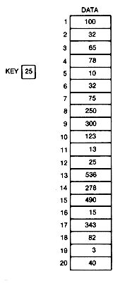
Figure 8.1 An Array of Integers to Be Searched for the Key Value 25
#define MAX 100
typedef struct
{int key;
}record;
typedef record recordarray[MAX];
linearsearch(data,n,key,pfound,ploc)
/* Searches the n records stored in
the array data for the search key.
Found will be true only if a record
is present with key field equal to
the search key value and then loc
will contain its array index.
*/
recordarray data;
int n,key,*pfound,*ploc;
{*ploc = 1;
while ((*ploc <= n) && (data[*ploc].key != key))
(*ploc)++;
*pfound = (*ploc < n + 1);
}
8.2.2 Saving Time: A Neat Trick
 n) for the end of the array before checking the next element. This is true whether the implementation is a for loop or a while loop. However, it is possible to avoid performing this test.
#define MAX 100
typedef struct
{int key;
}record;
typedef record recordarray[MAX];
linearsearch(data,n,key,pfound,ploc)
/* Searches the n records stored in
the array data for the search key.
Found will be true only if a record
is present with key field equal to
the search key value and then loc
will contain its array index.
*/
recordarray data;
int n,key,*pfound,*ploc;
{*ploc = 1;
data[n + 1].key = key;
while (data[*ploc].key != key)
(*ploc)++;
*pfound = (*ploc < n + 1);
}
8.2.3 Binary Search
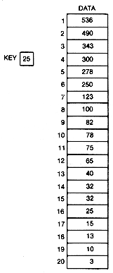
Figure 8.2 Array of Integers Sorted in Decreasing Order
#define TRUE 1
#define FALSE 0
#define MAX 100
typedef struct
{int key;
}record;
typedef record recorddarray[MAX];
binarysearch(data,n,key,pfound,ploc)
/* Searches the n records stored in order by
key field value(largest first) in the array
data for the search key. Found will be true
only if a record is present with key field
equal to the search key value and then loc
will contain its array index.
*/
recordarray data;
int n,key,*pfound,*ploc;
{int top, mid,bottom;
top = 1;
bottom = n;
*pfound = FALSE;
*ploc = 0;
while ((top <= bottom) && !(*pfound))
{mid = (top + bottom)/2
if (data[mid].key == key)
{*pfound = TRUE
*ploc = mid;
}
else if (data[mid].key < key)
bottom = mid - 1;
else
top = mid + 1;
}
}
8.2.4 Timing the Binary Search
 lg n
lg n times. If n is 20, for example, then 1g 20 = 4.32, and
  4.32
4.32 is 5. Thus in the worst case, the binary search is O(1gn). If each record stored is searched with equal frequency, then the average time to find a stored record is actually about (1g n) - 1.(The proof is not given here.)
8.2.5 Interpolation Search
8.2.6 Efficiency Comparisons
8.3: Elementary Sorts
8.3.1 Maximum Entry Sort
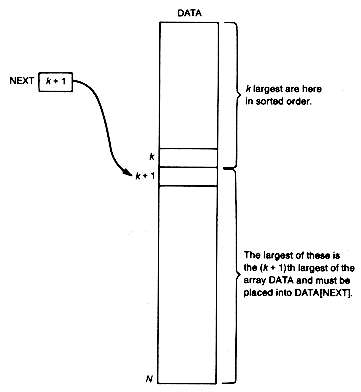
Figure 8.3 Ready to Determine the Next Largest
#define MAX 100
typedef struct
{int key;
}record;
typedef record recordarray[MAX];
maxloc (data,next,n)
/* Returns the array index of the
largest entry in data between the
entries indexed by next and n.
*/
recordarray data;
int next,n;
{int largest,i,tmaxloc;
tmaxloc = next;
largest = data[next].key;
for (i = next + 1; i <= n; i++)
if (data[i].key > largest)
{tmaxloc = i;
largest = data[i].key;
return (tmaxloc);
}
}
maxentrysort (data, n)
/* Sorts the n records stored in array data
in descending order.
*/
recordarray data;
int n;
{int next, loc;
for (next=1; next<=n - 1; next++)
{loc = maxloc (data,next,n);
interchange (data, next, loc);
}
}
interchange (data, i, j)
/* Interchanges the entries of
array data indexed by i and j.
*/
recordarray data;
int i,j;
{record tempdata;
tempdata.key = data[i].key;
data[i].key = data[j].key;
data[j].key = tempdata.key;
}
8.3.2 Bubble Sort

(a) Initial Array

(b) After Pass 1
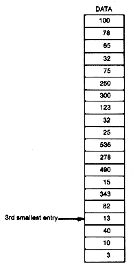
(c) After Pass 2
Figure 8.4 Bubble Sort
#define TRUE 1
#define FALSE 0
#define MAX 100
typedef struct
{int key;
}record;
typedef record recordarray[MAX];
bubblesort (data, n)
/* Sorts the n records stored in array data
in descending order.
*/
recordarray data;
int n;
{int i,done;
done = FALSE;
while (!done)
{done = TRUE;
for (i=1;i<=n-1;i++)
if (data [i +1].key > data [i].key)
{interchange (data, i, i + 1);
done = FALSE;
}
}
}
8.3.3 Timing the Bubble Sort
 (n - k) interchanges and comparisons. This sum is (n - 1) + (n - 2) +

 + 1 or [n(n - 1)]/2 interchanges and comparisons. The worst-case time for the bubble sort is O(n2), just as for the maximum entry sort. However, the maximum entry sort will always take time O(n2), since the number of comparisons it makes is not dependent on the data. The time taken by the bubble sort thus varies from O(n) for sorted data to O(n2) for reverse sorted data. The more ordered the initial data, the shorter the time.
8.3.4 Insertion Sort
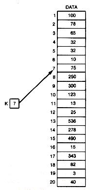
(a) Before Processing Record 7
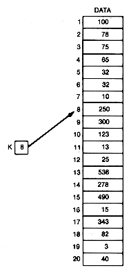
(b) After Processing Record 7
Figure 8.5 Insertion Sort
#define TRUE 1
#define FALSE 0
#define MAX 100
typedef struct
{int key;
}record;
typedef record recordarray [MAX];
insertionsort (data, n)
/* Sorts the n records stored in array data
in descending order.
*/
recordarray data;
int n;
{int k, i, inserted;
for (k=2;k<=n; k++)
{i = k;
inserted = FALSE;
while ((i > 1) && !inserted)
if (data[i - l].key < data[i].key)
{interchange(data,i,i - 1);
i--;
}
else
inserted = TRUE;
}
}
8.3.5 Timing the Insertion Sort


 + (n - 1) comparisons, plus the time for the 1 + 2 +

 + (n - 1) shifts down. Consequently, the total time is O(n2). This represents the worst case. Again we see that the time can vary with n2 for large n. The insertion sort, like the bubble sort, performs better the closer the initial data is to being sorted. If each of the n! possible initial orderings of the array with n distinct entries is equally likely to occur, then the average time for all three of the sorts considered so far is also O(n2).
8.3.6 Attempted Improvements


 + (n - 1) comparisons to 1g 2 + 1g 3 +

 + 1g (n - 1), which is about n 1g n. It does not, however, alleviate the need for the 1 + 2 +

 + (n - 1) shifts due to the insertions, so the time is still O(n2).

 + (n - 1) or [n(n - 1)]1/2 insertion time is reduced to time O(n). The list, coupled with the binary search reduction in comparison time to n 1g n, seems to give a new implementation of the insertion sort with worst-case time n 1g n. The fly in this ointment is that the ability to do a binary search has disappeared. It is no longer possible to locate the middle record by selection, which is what makes the binary search with sorted arrays so fast. Just the first record's location is known; the middle record can be found only by traversing the list and counting records until the middle one is reached.
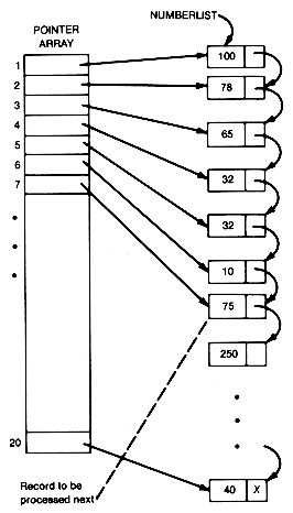
Figure 8.6 Selection of Records by Means of a Pointer Array
8.4: Heapsort: A Faster Sort
8.4.1 Heapsorts
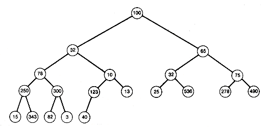
Figure 8.7 Not a Heap
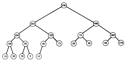
(a) A Heap
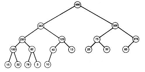
(b) After Removing 536 and Reheaping
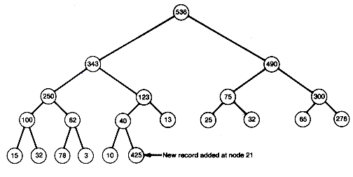
(c) After Adding a New Record to Heap (a)
Figure 8.8 Heaps
8.4.2 Creating a Heap
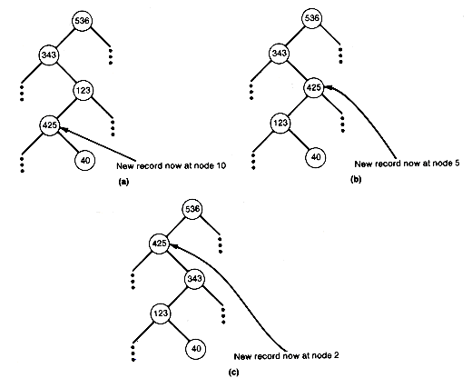
Figure 8.9 Heap Creation
8.4.3 Timing the Heap Creation
d =
 lg2(n + 1)
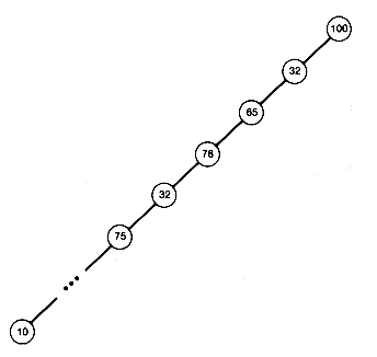
Figure 8.10 An Incomplete Binary Tree
 , where n is the number of nodes at depth k, d is the depth, and k is the number of comparisons and interchanges required for each node at depth k. This is because every record will work its way to the root of the tree when it is processed. Since nk = 2k-1, this sum will be proportional to n lg n. The efficiency of this method can be increased somewhat by first determining where a record to be processed will end up along its path to the root, and then shifting everything down before inserting it. This efficiency could also have been achieved with the insertion sort.
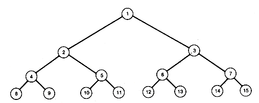
Figure 8.11 Binary Tree with Numbers Forming an Increasing Sequence
8.4.4 Better Heap Creation
 n/2
n/2 , the integer part of n/2, the first nonterminal node at depth d - 1. Process each node in turn, from node
  n/2
n/2 to node 1. The processing at each node i is to turn the tree with node i as its root into a heap. This can be done, assuming that its left and right subtrees are already heaps, as in the following example.
 11/2
11/2 ) (83 is stored there) and compare its successors 94 and 7, determining that 94 is the larger. Compare 94 with 83; since 94 exceeds 83, interchange 94 and 83 to obtain Figure 8.12(b).
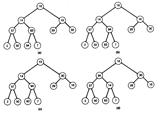
Figure 8.12 A Fast Heap Creation
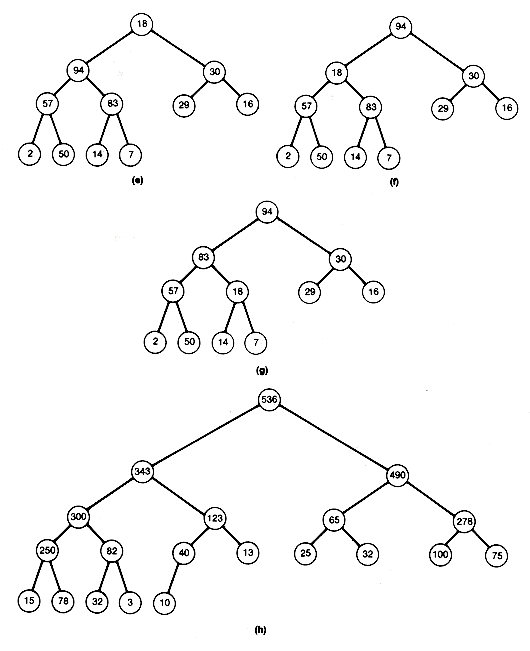
Figure 8.12
8.4.5 Some Details of Heap Implementation
8.4.6 Reheaping
8.4.7 An Implementation for Heapsort
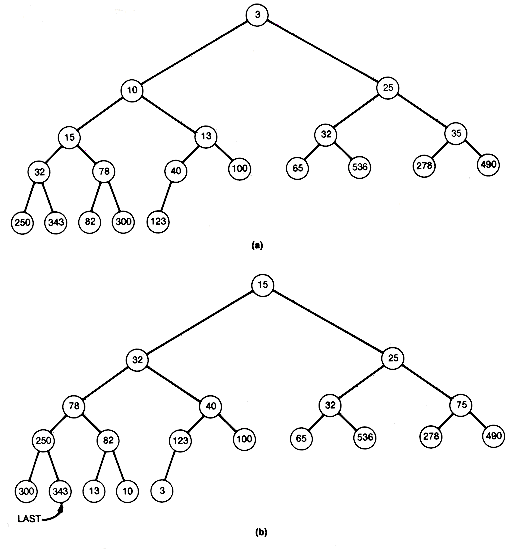
Figure 8.13 (a) Initial Heap and (b) Heap after First Three Entries Have Been Output
#define MAX 100
typedef struct
{int key;
}record;
typedef record recordarray[MAX];
heapsort (data,n)
/* Sorts the n records stored in array data
in descending order.
*/
recordarray data;
int n;
{int root,last;
root = n/2;
last = n;
while (root > 0)
{shift(data,root,last);
root--;
}
root = 1;
while (last > 1)
{interchange(data,1,last);
last--;
shift(data,root,last);
}
}
shift (data,root,last)
/* Makes the subtree of root into
a heap (min heap). The left and
right subtrees of root must be
heaps. All subtrees are stored
in array data in sequential
representation. Only the nodes
between root and last are
considered to be in the subtrees.
*/
recordarray data;
int root,last;
{int ptr,succ;
int keyvalue;
record recordvalue;
ptr = root;
succ = 2 * ptr;
if (succ < last)
if (data[succ + 1].key < data[succ].key)
succ++;
keyvalue = data[root].key;
copy(&recordvalue,&data[root]);
while((succ <= last) && (data[succ].key < keyvalue))
{copy(&data[ptr],&data[succ]);
ptr = succ;
succ = 2 * ptr
if (succ < last)
if (data[succ + 1].key < data[succ].key)
succ++;
}
copy(&data[ptr],&recordvalue);
}
8.4.8 Heapsort is Uniformly Fast
8.5: Quicksort: Another Fast Sort

Figure 8.14 Sorting an Array by Component
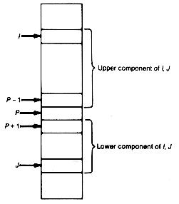
Figure 8.15 Array with a Partitioning Entry P Separating Upper and Lower Components
8.5.1 Two Quicksort Procedures
quicksort(i,j)
/* Sorts the records stored in array data
between positions indexed by i and j in
descending order.
*/
int i,j;
{int p;
if(i < j)
{p = partition(i,j);
quicksort(i,p-1);
quicksort(p+1,j);
}
}
quicksort(i,j)
/* Sorts the records stored in array data
between positions indexed by i and j in
descending order.
*/
int i,j;
{int p,top,bottom;
stack s;
setstack(&s);
push(j,&s);
push(i&s);
while(!empty(&s))
{pop(&s,&top);
pop(&s,&bottom);
while(top < bottom)
{p = partition(top,bottom);
if((p - top) > (bottom - p))
{push(p-l,&s);
push(top,&s);
top = p + l
}
else
{push(bottom,&s);
push(p+1,&s);
bottom = p - 1;
}
}
}
}
8.5.2 The Partition Function
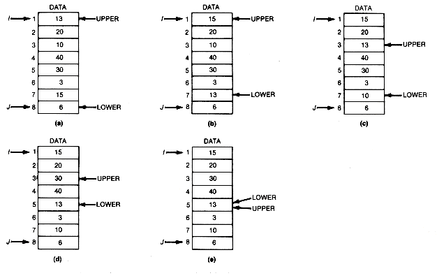
Figure 8.16 Sorting an Array by Means of a Partitioning Function
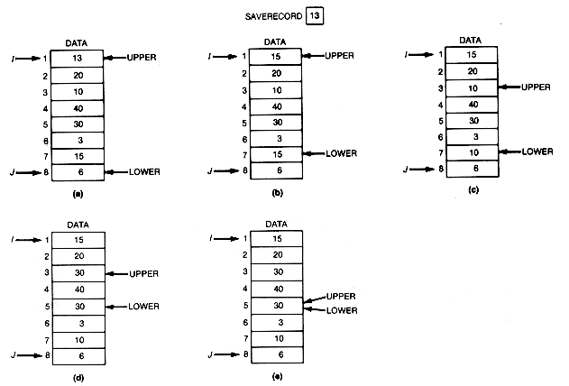
Figure 8.17 Partitioning an Array by Means of a Temporary Variable, SAVERECORD
partition(i,j)
/* Rearranges the entries in array
data between positions indexed by
i and j and returns an array index
which guarantees that all entries
above it are larger than the entry
it indexes, and all entries below it
are smaller.
*/
int i,j;
{int upper,lower;
record saverecord;
upper = i;
lower = j;
copy(&saverecord,&data[i]);
while(upper != lower)
{while((upper < lower) && (saverecord.key >=
data[lower].key))
lower--;
if(upper != lower)
copy(&data[upper],&data[lower]);
while((upper < lower) && (saverecord.key <=
data[upper].key))
upper++;
if(upper != lower)
copy(&data[lower],&data[upper]);
}
copy(&data[upper],&saverecord);
return(upper);
}
8.5.3 Analyzing Iterative Quicksort
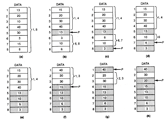
Figure 8.18 Iterative Quicksort
 bottom), the inner loop is exited. Unless the stack is empty, the outer loop removes the next problem from the stack, and the inner loop then functions again. Consequently, each entry that is placed in its proper position requires, at most, an execution of the inner loop body or an execution of the inner loop body plus the additional constant time required by the outer loop test plus removal of a problem from the stack. This means that the total time is, at most, c1 + c2 x n plus the total time taken by partition, for some constants c1 and c2.
8.5.4 The Worst and Best Cases
8.5.5 Distributive Partitioning
8.6: Simulation of an Algorithm
n = 40
-------------
Input Class Min Ave Max
------------------------------------
"Nearly sorted" int1 * * *
int2 * * *
comp1 * * *
comp2 * * *
"Random" int1 * * *
int2 * * *
comp1 * * *
comp2 * * *
"Nearly reverse int1 * * *
sorted" int2 * * *
comp1 * * *
comp2 * * *
 100
100 25,
25,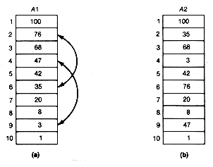
Figure 8.19 Array (b) Obtained from Sorted Array (a) by Two Interchanges
8.7: Simulation Results for the Sorts
8.8: Synopsis of Search and Sort Efficiencies
Table 8.1 Simulation Results in Actual Execution Time (milliseconds)*
n Bubble Sort Insertion Sort Modified Insertion Sort
-----------------------------------------------------------------------------------------------------------
10 1 2 6 8 9 1 2 5 7 7 0 2 4 6 9
20 1 8 23 33 36 1 5 16 28 30 1 6 17 25 30
40 2 31 101 138 148 2 16 67 110 121 5 16 65 107 120
100 4 217 646 863 923 7 89 412 678 761 6 87 402 660 744
200 8 966 2653 3463 3724 12 364 1657 2706 3058 11 354 1612 2639 2993
400 17 3933 11277 14732 15858 24 1583 7645 12489 14595 20 1373 6352 10581 12157
-----------------------------------------------------------------------------------------------------------
srt'd half rnd'm half rev srt'd half rnd'm half rev srtd half rndm half rev
srt'd rev srt'd srt'd rev srt'd srt'd rev srt'd
half srt'd half srt'd half srt'd
rnd'm half rnd'm half rnd'm half
rnd'm rnd'm rnd'm
n Heapsort Iterative Quicksort Recursive Quicksort
-----------------------------------------------------------------------------------------------------------
10 9 9 8 8 7 10 9 9 8 10 5 5 3 3 4
20 18 19 18 18 15 21 19 15 17 23 13 11 10 11 14
40 43 43 41 40 37 51 47 33 38 55 35 31 21 25 36
100 130 126 122 119 115 196 171 94 106 202 156 133 65 74 158
200 291 282 277 264 256 626 521 202 231 633 581 484 149 169 602
400 640 624 610 587 572 2175 1750 432 492 2195 2042 1644 318 372 2056
-----------------------------------------------------------------------------------------------------------
srt'd half rnd'm half rev srt'd half rnd'm half rev srtd half rndm half rev
srt'd rev srt'd srt'd rev srt'd srt'd rev srt'd
half srt'd half srt'd half srt'd
rnd'm half rnd'm half rnd'm half
rnd'm rnd'm rnd'm
-----------------------------------------------------------------------------------------------------------
Exercises
Suggested Assignments


