In this chapter the focus is on achieving efficient search and efficient insertions and deletion. Sometimes traversals through the data in sorted order by key value are also desirable. Four data structures that are appropriate for dealing with dynamic data are presented. First, priority queues are discussed. They provide the means to deal with a special case of insertion and deletion, as well as serving as an application of heaps. Next, hash tables are considered. Hash tables are important data structures that have excellent average search, insertion, and deletion times. Finally, binary search trees and AVL trees are introduced. These data structures support all the operations--search, insertion, deletion, and traversal--quite well.
9.2: Priority Queues
It often happens that there are a number of tasks, n, each with an associated priority. The n tasks are to be carried out in order of priority. When studying for examinations, most students review and prepare in an order of priority determined by the date of the exam. Most people read the chapters of a book in order, with priority determined by chapter numbering. In this case the situation is static, since the number of chapters does not change. Computer centers process submitted programs by attaching a priority to each and processing them in order of priority. Here the number of programs does change. This represents the usual case, where it is necessary to add new tasks with their priorities to the current collection. The general situation is covered by a priority queue.
A priority queue is a data structure with objects, their priorities, and two operations, insertion and deletion. Insertion in a priority queue means that an object with its priority is added to the collection of objects. Deletion from a priority queue means that an object with highest priority is deleted from the collection. A stack may be thought of as a priority queue with the highest priority object the one most recently added. A queue may be thought of as a priority queue with the highest priority object the earliest added.
High-level programming languages do not have priority queues directly available in their memories. It is important to be able to implement such queues, because they are of use in their own right and (as will be shown later) often appear as components of algorithms.
To implement a priority queue, first represent its objects and priorities as records with priority fields. Two ways to store the records come immediately to mind. The records can be stored in an array or in a list. In either case, the programmer may choose to store the records in arbitrary order or in order of priority. Table 9.1 gives the worst-case insertion and deletion times for each of the four resultant implementations, when n records are present in the priority queue. For example, when using the ordered array implementation, the top array record will have highest priority; thus deletion can be performed in constant time by using a pointer top to the current top record. Insertion of a record requires a search of the array to find its proper position. A binary search will allow this position to be found quickly, but to insert it requires O(n) time, because all records below it must be shifted down.
The table shows that if insertions are more frequent than deletions, it is better to use unordered records. In addition to considering the time for insertion and deletion, the amount of storage required for the list and array implementations must be evaluated. Arrays take less storage.
Another way to implement a priority queue is to use a heap. You have seen how to build a heap efficiently so that storage is minimal, heap creation takes at most O(n) time, and reheaping takes at most O(lg n) time. To use a heap for the priority queue, the records are stored at the nodes of a heap that is ordered by priority field values. To insert a new record, place it as a new rightmost entry at the greatest depth of the heap. Then let it work its way up in the heap as in the first heap creation algorithm. Adding the new record in this way will take time at most O(lg n). To delete a record, simply delete the record at the root of the heap, and then reheap by invoking shift. This takes time at most O(lg n). The time to create the heap initially will be at most O(n) if the second heap creation algorithm is used. This is also the time that would be required to create an initial unordered array or unordered list of records. To create sorted arrays or lists takes time at most O(n lg n). Referring to Table 9.1, you can see that the heap implementation affords a compromise solution. With arrays and lists, one operation can be done quickly (in constant time) and the other in O(n) time. With the heap, both operations can be done in at most O(lg n) time.
Still another way to implement a priority queue is as a leftist tree, which is a null binary tree or a binary tree with the following properties:
1. It is a heap.
2. Its left and right subtrees are leftist trees.
3. The path that is obtained by starting from the root and branching to the right until a node with no right successor is reached is the shortest path from the root to any node with at most one successor.
For example, the tree (a) of Figure 9.1 violates condition 3, while the trees (b) and (c) are leftist trees.
As an exercise, you should prove by induction on the number of nodes, n, in a leftist tree, that the shortest path in the tree, from the root to a node with at most one successor, contains at most
Leftist trees are implemented using a linked representation. (See Figure 9.2) Each node's record has an additional field, the distance field, containing the number of nodes along the right chain.
A leftist tree implementation of a priority queue has a number of pluses. Both additions and deletions can be done in constant time when the priority queue is acting as a stack. The time for these operations is O(lg n) for the general case. Also, two priority queues can be merged into one in O(lg n) time, where n is the total number of entries in the two priority queues to be merged. This is significantly faster merging than can be done with any of the previous methods, except for unordered lists. Crane [1972] introduced leftist trees as a data structure that can be used to implement priority queues. (See Knuth [1973b] for more details.)
The algorithm for merging two priority queues represented as leftist trees in O(lg n) time is as follows:
1. Make node.p the root of the merged tree, and merge q with p's right subtree.
2. Update the distance field of node.p.
3. If the distance of the root of the left subtree is not at least as great as the distance of the root of its right subtree, then interchange the two subtrees.
P is assumed to point to that root of the two leftist trees to be merged which contains the maximum key value, and q points to the other root. The result of merging the two trees p and q is shown as the tree r. The distance field values appear in parentheses. Notice in Figure 9.2 that, in effect, the two right chains of p and q are merged, with the other subtrees coming along for the ride. It is because only these two shortest paths participate in the algorithm that the time is O(lg n).
The next data structure we consider is the hash table. A hash table is a data structure for the storage of records. It provides a means for rapid searching for a record with a given key value and adapts well to the insertion and deletion of records. Many compilers, for example, use hash tables to implement their symbol tables. They are also used extensively in systems where the primary objective is information retrieval. Thus nametable of Chapter 6 or a dictionary of words might be implemented in a hash table.
To illustrate the need for hash tables, suppose we want to store 1,000 records representing 1,000 customer accounts. Assume that each record has an account number as its key and, since we control account numbers, they range from 1 to 1,000. The solution is simple. Store the record with key value i in element i of an array data. Then, given a key value to search for (say, 836), go directly to element 836 of data to find it. What could be a quicker search? We are given a record and know immediately where to go to find it. The search time is a constant, independent of the number of records stored. However, this kind of search requires the ability to assign key values so that all keys are within a range of array indices (1 to 1,000 in this case). It also requires that we have enough storage to accommodate all records.
Now suppose we are dealing with records representing information about our employees, and that the keys are social security numbers. Even with only 1,000 employees, there are 109 possible social security numbers. It is not possible to know in advance which of the 109 social security numbers our 1,000 employees will actually have. If we were to allocate storage using social security numbers as addresses, we would run into two problems. First, there would not be enough storage. Second, if we did have sufficient storage, 999,999,000 (109 - 103) storage elements would be wasted! Nonetheless, it is extremely attractive to be able to look at the search key value and to know where to find it. This is the goal of hash tables and hash searching--to find a record directly, given its key value.
This section deals with a scaled-down version of the social security example. There are eighteen records, each with a key value that is a three-digit number. The records and their key values will be given in some order, normally unpredictable. We are to build a table, implemented in an array, in which the eighteen key values will be stored, so that searching can be done efficiently. One way to do this is to build a special kind of table--a hash table. This table will then be searched for given key values. To build a hash table requires a hashing function and a collision resolution policy. A hashing function is a method of calculating an array or table address for any key. To be useful, the address must be quickly calculable.
The hash function should have other properties, as will become evident. The hash function used here assigns to any key the remainder after division of the key by the table size. If the table size is m and the key value is k, then k mod m denotes this remainder. The starting table or array size is 23.* The eighteen key values and their order are given in Table 9.2, along with the hashing function values assigned to each.
* With division-type hashing functions, the divisor, or table size, is usually a prime number greater than the number of entries to be placed in the table. We have taken this prime to be 23.
The hashing address for 019 is found, for example, by dividing 019 by the table size 23, to obtain 019 = 0 X 23 + 19. The remainder, 19, is the assigned hashing address. As each key value is input, its hashing address is calculated, and the key value is placed into that element of the table. After the first four key values are entered, the table is as shown in Figure 9.3(a).
When the fifth key value, 663, is input, its hashing address is 19, but element 19 of the table is already occupied by another key value. This event is called a collision. The collision resolution policy is the method used to determine where to store a value that has undergone collision. The most straightforward policy for resolving the conflict is called linear probing. It entails proceeding through the table from the collision element and placing 663, the colliding entry, into the first unoccupied element found. The hash table is assumed to have been initialized, so that each element was "unoccupied" or "empty." If the search for an empty element reaches the end of the table, it circles to the top of the table. In this case, 663 is entered at element 20. The final table is shown in Figure 9.3(b). A total of eight initial collisions occurred in building it.
Each time a location of the table is accessed in an attempt to insert a key value, one probe has been made. To enter the first key value required one probe; to enter the fifth key value required two probes. To enter keys 1 through 15 required, respectively, 1, 1, 1, 1, 2, 1, 4, 1, 1, 1, 2, 1, 5, 4, 7, 3, 1, 3 probes. You can build the table and confirm these probe numbers.
How would you search a hash table when asked to find a given key, such as 642? If the key were stored in the table, it would either be found at its hashing address or at the end of a linear probe. If its hashing address were empty, or if the search came to an empty element in the linear probe before finding the key, you might conclude that it was not stored in the table. In this case, the hash address of 642 is 21. Element 21 is not empty but does not have 642 as its value. If you do a linear probe, you will eventually come to element 3, which is empty, without finding 642; thus you would conclude that 642 is not in the table.
If the key searched for were 802, you could go to its hash address (20), find that element occupied with a different key, and start the linear probe, finding 802 at element 0.
Notice that if the search key value is present in the table, the search will require exactly as many probes to find it as were required to enter it into the table. The search traces out the same path. Instead, if the search is for a key value that is not present, the search will take exactly as many probes as would be required to enter it into the current table.
A search that finds a key value is called successful, and one that fails to find a key value is unsuccessful. Theoretically, one can calculate the number of probes required for every possible key value. Knowing the frequency with which each possible key value (there are 1,000 in our example) will be searched for, one can determine the average number of probes required to search the table. The maximum number of probes can always be determined given the table. In the example, a successful search would require at most seven probes, while an unsuccessful search (for example, for key value 248) could require nine probes. If one never had to search for a key not stored, and all stored keys were searched for with equal frequency, the average number of probes would be
or 40/18 = 2.22 probes. This calculation involves multiplying the frequency of search for each record by the number of probes required to enter it, and then adding all these products. In this case, each frequency was 1/18, and the required probes were noted when the hash table was built.
If no collisions occurred in building the table, every successful search would take exactly one probe. If the hash function actually assigned every key value not stored in the table to an empty address, exactly one probe would be required for any search. This would be the ideal situation. It is apparent now that a desirable hashing function will "scatter" or distribute the key values throughout the table, so that relatively few collisions ensue.
The hash table was of length 23 and stored eighteen key values. Its usage ratio is 18/23; the table is 78 percent full. Intuitively, the lower this ratio, the greater the storage wasted, but the lower the likelihood of a collision. Appropriate hashing functions must be selected with care in real applications, but it is possible to achieve very quick searches using hash tables.
A great deal of literature in computer science is devoted to the selection of hashing functions and collision resolution policies. To give some idea of what can be achieved, this section states results for an idealized scheme that assumes the hashing function to be perfectly random. Given any key value, the scheme assigns an address to that key value by picking randomly from among all the addresses of the table. This random selection is made so that each of the m addresses in a table of size m is equally likely to be selected. The table is built by inserting, in turn, each given key value. A key value is stored by determining its hash address. If that address is empty, the key value is stored there. If that address is occupied, the collision resolution policy works as follows. Another random hash function again selects an address at random. If that address is empty, the key value is stored there. If it is occupied, this procedure is repeated until the key value is finally entered. Thus an insertion of a key value may require the generation of a sequence of hash addresses ending with the actual final storage address.
After the table is built, searches are performed as follows. Trace the sequence of hash addresses that were generated to store the search key (if it is in the table) or that would have been generated (had the key been stored). The basic assumption made here is that the hash functions generate precisely the same sequence of hash addresses for the search as for building the table. This may seem like a strange way for random hash functions to work, but it is our assumption nevertheless. Table 9.3 shows the theoretical results for such a scheme, when n keys are stored in the table of size m.
The successful and unsuccessful search columns are given approximately by the functions (1/
Hash tables are not a searching panacea. A major disadvantage is that entries will not be in order by key. The only way to access the records in sorted order is to sort them. However, if this isn't important, hashing is often a good approach.
The linear probing collision resolution policy is a special case of open addressing. The idea of open addressing is to resolve collisions by following a specific probe sequence whenever a collision occurs, in order to determine the insertion location for a new key. To be specific, let ki denote the key stored in the ith location of a hash table of size m. Assume that at least one table location is unoccupied and set all unoccupied locations to the "null" key value. This prevents "falling off" the table when searching for a key and reduces the search time, because an end-of-table search test need not be made.
Let h(k) denote the hash function value for search key k. The sequence of indexes determined by
[h(k) + i X p(k)]mod m* for i = 0, 1, 2, . . . , m - 1
is a probe sequence if the indexes are all distinct. This implies that, as i goes from 0 to m - 1, the generated indexes form a permutation of the indexes 0, 1, 2, . . . , m - 1. Consequently, in attempting a new key insertion, all locations of the hash table will be accessed in some order before deciding that the key cannot be inserted. It also ensures that, in attempting to search for a key, all locations of the table will be accessed in some order before concluding that the search key is not in the table, or until a null key is encountered.
* The formula states that the ith index in the probe sequence is found by calculating [i + p(k)]mod m. However, if the previous index, the (i - 1)th, is known, then simply adding p(k) to it and taking the result mod m will also yield the ith index.
Linear probing is the special case obtained by taking p(k) = 1 for all keys k. In general, a key is inserted by accessing the table locations given by its probe sequence, determined by [h(k) + i X p(k)]mod m as i goes from 0 to m - 1, until a null key is encountered. The key is then inserted in place of that null key. A search is done the same way. The algorithm for a hash table search using a probe sequence is as follows:
1. Set i to h(k)
2. While ki is not the search key k and ki is not the null key
set i to [i + p(k)]mod m.
3. If ki = k, then
set found to true
else
set found to false.
Notice that p(k) represents a displacement from the current probe address.
With linear probing, large clusters of keys stored in adjacent locations of the hash table tend to get larger as insertions are made. This is because large clusters have a greater probability of the new keys' hash address falling within the cluster, assuming a "random" hash function and "random" keys. A cluster gets larger when a new key is inserted at either end of the cluster, or when two separated clusters become connected because of the new key insertion. Both of these events occurred in the scaled-down social security number example. This phenomenon is called primary clustering. As the table usage ratio increases, primary clustering leads to greater search and insertion times. This is clearly undesirable. It happens because the large clusters must be traversed, with the average time being proportional to half the cluster length when keys are searched with equal frequency. Thus the insertion, or search for a key, begins to look like a linear search through a cluster.
To avoid primary clustering, try taking the next probe to be in a position removed from the current one instead of being adjacent to it. This is open addressing with displaced linear probing. Taking p(k) =
7, 12, 4, 9, 1, 6, 11, 8, 0, 5, 10, 2
Note that any key k whose hash address is 7 will have exactly the same probe sequence. Even worse, suppose a key's hash address is 11, and 11 is occupied upon its insertion. The next probe for this key will be in location [11 + 1 X 5] mod 13, which is location 3. A collision at 3 will result in a further probe at [3 + 1 X 5] mod 13 or 8, then 0, 5, etc. Thus the key that originally hashed to address 11 picks up at the intersection of 11 with the probe sequence for any key hashing to 7, and follows that same probe sequence from 11 onward. Similarly, any key that collides, upon insertion, with a key already occupying its hash address, will continue along this exact probe sequence from its point of entry.
In effect, there is exactly one probe sequence for all keys; they just enter, or merge into it, at different positions specified by their hash addresses. This means that, as a "cluster" builds up along this probe sequence (say, at 11, 3, 8, 0, and 5, as they become occupied), it has the same tendency to grow as a cluster of physically adjacent occupied addresses did with linear probing. This is just primary clustering, although the clusters do not appear in adjacent locations.
We need effective techniques for dealing with this problem. Figure 9.4 gives the hash tables that result from their application to our example. The hash tables produced by linear probing, and the displaced linear probing just discussed, appear in tables (a) and (b) of the figure, corresponding to
The average number of probes for a successful search of this table is 1/18 X (11 X 1 + 5 X 2 + 1 X 3 + 1 X 12) = 36/18 or 2.00, which is an improvement over linear probing for this example. However, for the reasons stated previously, the theoretical average number of probes in a successful search will be the same as for linear probing.
How can we eliminate or break up large clusters to improve these results? It can be done using open addressing with secondary clustering. Consider the following analogy. Suppose there are m stores, each selling a certain specialty item, and each with exactly one such item in stock. Assume n people decide to buy that item the same day, and they, in turn, each select one of the m stores at random. If a customer finds the item in stock at the shop of his or her choice, he or she buys it. However, if someone has already bought the item, it will be out of stock, and the person may ask the store manager for directions to another store. Let the stores be numbered from 0 to m - 1. Whenever this occurs, suppose the manager of the ith shop sends the customer to the (i + 1)th shop. Of course, the manager of the (m - 1)th store refers people to the 0th store. The result of all this feverish activity is that all customers arriving at a particular out-of-stock store are sent to the same next store. Again, at that store, they are all sent to the same next store whenever the item has been sold. It seems clear that this results in primary clusters of customers being formed. The physical locations of the stores is irrelevant to this process.
Suppose each store manager, instead of giving identical directions to each would-be purchaser, sends customers to another store depending on which store they tried originally and on the number of stores they have already been to. The effect will be to disperse the unhappy customers. Rather than all these people being sent on to the same sequence of shops, only those with the same initial shop and the same number of previous attempts at buying are given identical directions. Clusters should still appear, but they should tend to be smaller than the primary clusters. This is, in fact, what happens, and the clusters that appear after such dispersion are called secondary clusters.
Translating this remedy to the problem involves choosing p(k) so that it becomes a function of h(k), the initial hash address of key k. This implies that only keys hashing to the same address will follow identical probe sequences. Unlike linear or displaced linear probing, keys whose probe sequences intersect do not merge into the same probe sequence at intersection. They go their separate ways. Again, to ensure that p[h(k)] generates a probe sequence, it is necessary to choose it carefully. As long as p[h(k)] is not a factor of m, for each key k, a probe sequence will result. If m is a prime number, this will always be the case when p[h(k)] is between 0 and m - 1.
As an example, take
Using our h(k) = k mod m and m = 13, any key with hash address 7 (say, key 137) has the probe sequence
7, 5, 3, 1, 12, 10, 8, 6, 4, 2, 0, 11, 9
Any key hashing to 11 now (say, key 258) has the probe sequence
11, 0, 2, 4, 6, 8, 10, 12, 1, 3, 5, 7, 9
Notice that a collision at 11, for such a key, does not result in the probe sequence for keys with hash address 7 being followed from its intersection with 11. It follows the sequence 11, 0, 2, . . . instead of 11, 9, 7, 5, . . . .
The hash table for this secondary clustering remedy is hash table (c) of Figure 9.4. The average number of probes for a successful search in this table is 1/18 X [(11 X 1) + (3 X 2) + (3 X 3) + (1 X 5)] = 31/18 or 1.72. This gives an improvement over hash tables (a) and (b), as expected. It occurs because the secondary clusters tend to be shorter than the primary clusters. Notice that the "physically adjacent" clusters in the table are deceiving; they are not relevant. It is the clustering along the probe sequences that is important. In linear and displaced linear probing there is, in effect, only one probe sequence. With the secondary clustering techniques, there is a distinct probe sequence for each distinct hash address.
Open addressing with the quadratic residue technique attempts to break up primary clusters in a similar way, although it generates a probe sequence somewhat differently. The probe sequence for key k starts with h(k) and follows with
[h(k) + i2]mod m, [h(k) - i2]mod m for i = 1, 2, . . . , (m - 1)/2
Again, to ensure that m distinct indexes are generated, care must be taken in the choice of m. If m is prime and of the form (4 X j) + 3, then m distinct indexes are guaranteed. Since m = 23 in our example, j = 5 and (m - 1)/2 = 11. The probe sequence for key k is then
h(k),
[h(k) + 12] mod 23, [h(k) - 12] mod 23,
[h(k) + 22] mod 23, [h(k) - 22] mod 23, . . . ,
[h(k) + 112] mod 23, [h(k) - 112] mod 23
If k is 364, h(k) = 19, and the probe sequence is
19, 20, 18, 0, 15, 5, 10, 12, 3, 21, 17, 9, 6, 22, 16, 12, 1, 8, 7, 4, 11, 2, 13
This is really a secondary clustering technique, since keys that hash to the same address will still have identical probe sequences. The hash table for this technique appears as hash table (d) of Figure 9.4, which gives an average number of probes of 1/18 X [(10 X 1) + (4 X 2 ) + (3 X 3) + (1 X 4)] = 31/18 or 1.72 for a successful search. When a key is inserted with these secondary clustering techniques, the result may be the lengthening or connecting of two clusters. These events may occur simultaneously along more than one probe sequence when the key is inserted.
Returning to the example of the out-of-stock specialty item, we might look for a remedy that avoids even these secondary clusters, since they also tend to increase search and insertion times. It seems reasonable to try to disperse these secondary clusters by giving each would-be customer a seperate set of directions. This may be done by having store managers randomly select the next store for a customer to try. This idea is known as open addressing with double hashing. The technique uses a second hash function for p(k). To be most effective, this should be as "random" as the initial hash function and should assign a value to key k by selecting this value independently of the value assigned to key k by the initial hash function.
The theoretical analysis for this technique has not been carried out as fully as for other methods, but the results indicate that double hashing gives the best results among the open addressing techniques. Empirically, it gives results that are the same as those for "random" hashing (see Table 9.3). This is somewhat suprising, since random hashing corresponds to our store remedy. Double hashing, instead of picking a store randomly, over and over again, until a customer is satisfied, merely picks an individual displacement at random for each key. This displacement then determines the probe sequence for a given hash address.
Care must be exercised in the selection of the second hash function so that a desirable probe sequence is generated. If m is a prime, then one possibility that ensures the generation of such a probe sequence is
For instance, p(657) = 11, since 657 = 50 X 13 + 7 when m = 13. Hence the probe sequence for 657 is
7, 5, 3, 1, 12, 10, 8, 6, 4, 2, 0, 11, 9
Key 137 also has hash address 7, but p(137) = 10, since 137 = 10 X 13 + 7. Its probe sequence, however, is distinct from 657's:
7, 4, 1, 11, 8, 5, 2, 12, 9, 6, 3, 0, 10
Now, even keys with the same hash address are unlikely to have the same probe sequence. The idea is that, statistically, probe sequences should appear to be approximately independently and randomly generated for two distinct keys. The hash table produced by this technique is given as hash table (e) of Figure 9.4, and the average number of successful probes is 1/18 X [(11 X 1) + (4 X 2) + (2 X 3) + (1 X 4)] = 29/18 or 1.61
As a further illustration, suppose key 582 is to be inserted in the hash tables of Figure 9.4. Its hash address, 582 mod 23, is 7, since 582 = 25 X 23 + 7. The sequence of probed locations and the number of probes required for each table are given below.
It is interesting that the average number of probes required to make an insertion is the same as the average number of probes required to carry out an unsuccessful search. This fact is useful in the analysis of hashing. The results of the example are typical of the behavior of open addressing techniques. As the usage ratio of the table increases, the secondary clustering and quadratic residue methods provide considerable improvement over the primary clustering methods. The double hashing techniques improve the results even more. For lower usage ratios, the improvements are much less noticeable. These improvements in average numbers of probes do not translate directly into similar improvements in average times, which depend on implementation details.
Chaining is another method of collision resolution. The idea is to link together all records that collide at a hash address. These may be kept separately or within the hash table itself. Separate chaining treats each location of the hash table as the head of a list--the list of all keys that collide at that location. Separate storage is used to store records of the list, which consist of key values and link pointer values. When a collision occurs, an insertion is made at the front of the corresponding list. Using this technique for our example yields the hash table shown in Figure 9.5 with corresponding numbers of probes (key comparisons). The table's average number of probes for a successful search is 1/18 X [(12 X 1) + (5 X 2) + (1 X 3)] = 25/18 or 1.39.
In contrast to open addressing, separate chaining allows clusters to form only when keys hash to the same address. Hence the lenghts of the lists should be similar to the lengths of clusters formed with secondary clustering techniques. A comparison of the 1.39 probes to the 1.89 or 1.72 probes with secondary clustering is somewhat unfair, since the hash table with separate chaining really uses additional storage. The actual amount of additional storage depends on the record lenghts. When they are small, and storage that would otherwise be unused is available for the link pointer values, then the usage ratio should more properly be measured as n/(n + m). This is 18/41, or 44 percent, in the example. When the link field takes up the same amount of storage as a record, then the usage ratio should more properly be measured as n/(2n + m). This is 18/59, or 31 percent, in the example.
Coalesced chaining maintains lists of records whose keys hash to the same address. These lists are stored within the hash table itself. Whenever two such lists "intersect," they coalesce. This is analogous to two separated clusters becoming connected when a new key is inserted in the location that separated them. Each hash table entry is now a record containing a key value and a link value to the next record on its associated list.
A key is inserted into the table by going to its hash address and traversing its list until a null key is found, the key itself is found, or no records remain on the list. If the null key is found, the new key is inserted in the record stored at that location, and its link field is set to null. If the key itself is found, no insertion is necessary. If no records remain on the list, then an unoccupied location must be found, the new key inserted there, and its link field set to null. This new record must then be appended at the end of the traversed list.
In order to create this new record to be appended, a pointer p is kept updated. Initially, p points to location m (which is just off the table). Whenever a new record must be found, p is decremented by 1 until the location it points to is unoccupied. If p "falls off" the table (becomes less than 0), then the table is full and no insertion is possible.
Figure 9.6 illustrates coalesced chaining for the example. P is initially 23 and the first four keys are inserted directly into their hash addresses. Key 663 collides at its hash address, 19. P is then decremented by 1 and, since location 22 is empty, 663 and a null next pointer are inserted there. This new record is then appended at the end of the list beginning in 19, by setting the link field of location 19 to 22. Key 262 is inserted directly into its hash address, 09. The next entry is 639, but its hash address, 18, contains an entry. P is then decremented by 1, and since location 21 is empty, 639 and a null link value is inserted there. This record is then appended at the end of the list beginning in 18 by setting the link field of location 18 to 21.
Figure 9.6 shows the resultant hash table, the number of probes for each key insertion, and the value of p after all eighteen keys are entered. The average number of probes for a successful search of this table is 1/18 X [(9 X 1) + (6 X 2) +(1 X 3) + (1 X 4) + (1 X 5)] = 33/18 or 1.81. If extra storage is available for the link fields, then n/m is a reasonable measure of the table usage here. These 1.81 probes are not as good as the 1.61 or 1.72 probes resulting from double hashing and quadratic residues in the example. Theoretical results, however, show that coalesced chaining does yield better average results than "random" hashing when storage is available for link pointer fields. You may expect coalesced chaining to give results that are not as good as separate chaining, better than linear or displaced linear probing, not as good as "random" or double hashing, but perhaps comparable to the secondary clustering techniques. If the link fields take additional storage, it should be taken into account in the usage factors for comparison. Note that coalesced chaining generally yields more but shorter lists (or clusters) than linear or displaced probing, because connecting or coalescing of clusters occurs to a lesser extent with coalesced chaining.
A third method of collision resolution will be discussed in Chapter 10 in connection with external memory, or secondary storage, where it is especially appropriate and useful.
If keys are entered into a hash table in sorted order, open-addressing and chaining techniques will always result in searches along a probe sequence or along a list, in which the keys appear in the same or reverse order, respectively. In both cases, the search algorithm may be easily modified so that whenever a key is encountered that precedes the search key in the relevant ordering, the search is immediately terminated unsuccessfully. This can significantly decrease search times for unsuccessful searches but will not affect successful search times. You can generate the new hash tables (a) through (g) of Figures 9.4 to 9.6 to see the effect on the tables of the keys appearing in sorted order.
Of course, one cannot normally control the order in which keys to be inserted appear. It is not difficult, however, to modify the insertion algorithms so that the resultant hash table is exactly the same as the hash table resulting when keys are given in sorted order. The idea of the algorithm is clever and simple. For open addressing, simply insert a key as usual unless, in following a probe sequence, a key is encountered that precedes the new key in the ordering. Then the search key is inserted in that position, and the insertion proceeds as though the replaced key were being inserted using the displaced key instead of the new key. For separate chaining, it is necessary to traverse the list at which a collision occurs, and insert the new key in its proper position of the list.
This technique does not work directly for coalesced chaining, because the insertion of a new key in a list may start from the interior of the list when a collision occurs. In order to keep coalesced lists in order, it is necessary to find the first list record or be able to traverse the list in either direction. To achieve this, the lists might be implemented as circular lists or two-way lists. Circular lists take more traversal time but less storage than two-way lists.
Keeping ordered hash tables yields significant improvements in the average number of probes required for unsuccessful searches with open addressing. These improvements are especially striking for high usage ratios.
Deletion in hash tables using separate chaining is straightforward, since it amounts to the deletion of a record from a list. With open-addressing and coalesced chaining, the deletion of a key is not so straightforward, since a key of the table will be needed to reach another key when it is on that key's probe sequence or list. Deleting it would break this path. One solution to this problem is to mark a deleted key location as "deleted," so that the path is not broken. When a significant fraction of keys has been deleted, the actual usage ratio of the resultant table is low, but search times will still reflect the original higher usage ratio. New insertions, when encountering a "deleted" location, may recapture this wasted storage by occupying such "deleted" locations. However, if "deleted" locations build up, without being recaptured by insertions, search times deteriorate to a linear search for unsuccessful searches and are larger than necessary for successful searches. The only remedy is to rebuild the hash table. Although the algorithm is not given here, this may be done in place, by using only storage allocated to the table in order to carry out the creation of a new table. Hash tables can also be expanded or decreased in size, and recreated. Again, this can be done in place.
Let us review the advantages and disadvantages of hashing. First, note that some estimate is needed in advance for the maximum number of entries to be stored in a hash table, since its size must be declared. This is important; too high an estimate wastes space, and too low an estimate means a large usage ratio and poorer performance. Second, the hash function must be carefully chosen so that it can be computed quickly and generates relatively few collisions.
The main characteristic of hashing is its excellent average search, insertion, and deletion time. However, when deletions are frequent, care is required in deciding which collision resolution policy to use. The major disadvantages of hashing are the possibility of large worst-case times and the lack of support for traversal through the records in sorted order. Also, the only information obtained from an unsuccessful search is that the record isn't in the table. In the data structure considered next, more information may be obtained.
Choosing the appropriate hashing technique involves consideration of time and storage as well as the relative frequency with which successful searches, unsuccessful searches, and deletions will occur. However, some generalizations can be made.
Using open addressing to resolve collisions can be quite efficient for moderate usage ratios. Although the average times for successful searches depend on whether simple linear probing or more complex probing such as double hashing is used, the differences are small. These differences are more significant for unsuccessful searches, so more complex probing is desirable when they will occur frequently. Ordered hash tables can significantly reduce the search times in this case. For larger usage ratios the chaining methods have superior search times.
With open addressing, when deletions are frequent, the table can actually be storing relatively few entries, with many table positions simply marking deleted entries. Thus the table performance is governed by a usage ratio that does not reflect the actual, much smaller, number of positions used to store records. Separate chaining uses storage more efficiently in this case, and deletion is easy. Separate chaining also has better average time behavior than the other methods.
When records are small, the links required by chaining take significant extra storage compared to open addressing, whereas the opposite is true when records are large. When record size is moderate, the extra storage for links using separate chaining must be weighed against the reduced usage ratio that could be obtained if this storage were used in open addressing.
We turn now to the next data structure: binary search trees. A binary search tree is a binary tree with the property that its left subtree contains records no larger than the root record, its right subtree contains records no smaller than the root record, and its left and right subtrees are also binary search trees. This is a recursive definition.
A binary tree fails to be a binary search tree if even one node contains a record in its left subtree or its right subtree that is, respectively, larger or smaller than the record stored at the node. Figure 9.7 has three examples of binary search trees containing the same fifteen records.
Note that a binary search tree need not be a heap, and that a heap need not be a binary search tree. In general, they are different kinds of binary trees. There are many binary trees that can store the same records. Any binary tree with n nodes can store n records in such a way that the tree is a binary search tree. (Just do an inorder traversal of the binary tree and insert the records in sorted order.)
In Chapter 7, three important traversals through the nodes of any binary tree were defined: 1) preorder, 2) inorder, and 3) postorder. In order to search a binary tree to determine if a particular key value is stored, any one of those traversals could be used to gain access to each node in turn, and the node tested to see if the search key value is there. This would be equivalent to a linear search.
Instead, the special nature of binary search trees facilitates highly efficient search. We simply compare the search key with the root key. If they match, the search is complete. If not, determine whether the search key is smaller than the key at the root. If so, then if it is in the tree at all, it must be in the left subtree. If it is larger than the root key, it must be in the right subtree if it is in the tree at all. Thus either the left or right subtree is eliminated from consideration. This procedure is repeated for the subtree not eliminated. Eventually, the procedure finds the key in the tree or comes to a null subtree and concludes that the key is not stored in the tree.
Assume that nodes of the binary search tree are represented as follows.
This special search may be implemented as follows:
Found indicates whether the search key value was present in the tree. If so, p points to the node in which the search key was found, and pred points to its predecessor. If the search key was not found, then pred points to the node that would have been its predecessor had it been in the tree. Note that this allows additional information to be obtained, if desired, beyond the fact that the search key was not found. The key less than the search key and the key greater than the search key can easily be determined, so that records closest to the desired one are known.
Notice that when (b) of Figure 9.7 is searched in this way, the search is equivalent to a linear search of an array in which the records are stored in sorted order. This search algorithm, applied to (c), would be equivalent to a binary search of an array in which the records are stored in sorted order. A search of (a) would fall somewhere between these two extremes.
What allows the search of Figure 9.7(c) to be equivalent to a binary search? It is the fact that the tree is "scrunched up" or near minimum possible depth, and not as straggly (unnecessarily deep) as the others. It has an intuitive kind of "balance," so that we eliminate from consideration about half the records each time we make a comparison. We are back to the game of "twenty questions.''
This section develops an algorithm for creating or growing a binary search tree that stores records at its nodes. Imagine that you have already processed some records and created a binary search tree for them. Given the next input record, search the current tree for its key value. Assume no duplicates will occur in the tree, although this need not create any real problem, since a node can contain a pointer to a list, stored separately, of records with identical key values. Eventually, since the new record is not in the tree, a null subtree will be reached. However, if this null subtree is replaced by a node that stores this record, the resultant tree will still be a binary search tree. For instance, inserting 45 by this procedure in Figure 9.7(c) produces Figure 9.8. This gives an algorithm for growing a binary search tree. Start with the first input record at the root. For each additional input, search the tree. The search will reach a node whose left or right successor must be followed, but the successor is null. The record replaces that null subtree.
This can be accomplished by using pred from the search implementation, and then invoking the following.
We now have algorithms for growing, searching, and inserting records into a binary search tree.
The binary search tree grown by the algorithm of the preceding section will have its shape determined by the input order of the records to be stored. If they are input in sorted order or reverse sorted order, the result is Figure 9.7(b) or its mirror image. If they are input in the order 55, 40, 83, 35, 51, 80, 85, 17, 37, 50, 52, 70, 81, 84, 100, the result is Figure 9.7(c). There are n! possible input orderings of n distinct keys. Some of these may give rise to the same binary search tree. Recall that the tree grown cannot have depth greater than n nor less than
It is difficult to analyze this problem using probability theory. However, the average depth has been shown to be O(c lg n), where c is about 4. The average search time can be calculated for a randomly grown binary search tree. It is the average time required to search for a record stored in the binary search tree, assuming each record is equally likely to be searched. This average search time is O(1.39 lg n). In the case of random input, the average search of the binary search tree grown by the algorithm will be only 39 percent more than the smallest possible average search time! Moreover, the algorithm for growing the tree will take an average time at most O(nlg n). If the records are given in sorted order instead of in random order, it will take the algorithm O(n2) time to grow the tree.
It is possible to grow "balanced" binary search trees, also called AVL trees (after the discoverers of these trees, Adelson-Velskii and Landis [1962]). The algorithm for growing AVL trees is slower and more complex, as is the insertion and deletion of records. However, they are guaranteed to have depth no greater than about 1.44 lg n. This is the worst-case depth. Consequently, AVL trees may be searched in time at most O(1.44 lg n). Such trees appear quite healthy and are never sparse. However it takes great care to grow healthy trees, as will be seen later.
At this point all the important operations on binary search trees have been considered except deletion. The purpose of this section is to derive an algorithm for deleting a record from a binary search tree so that the remaining tree is still a binary search tree. To delete a terminal record, simply replace it by a null tree. To delete a record with only one successor, simply insert the successor's subtree at the position occupied by the deleted node. For instance, in the tree shown in Figure 9.9(a), deleting 51 and 71 yields the tree shown in Figure 9.9(b).
Consider Figure 9.9 again. A difficulty occurs if you wish to delete 80, a record with two successors. The node 80 must be replaced by a record that will allow the tree to retain its binary search tree property. This means that the record replacing 80 must be at least as large as any record in the left subtree of 80, and no larger than any record in the right subtree of 80. There are two choices: replace 80 with the largest record in its left subtree or the smallest record in its right subtree.
Notice that the largest record in any binary search tree is always found by going to its root and following right successors until a null tree is reached. The smallest record is found by going to its root and following left successors until a null tree is reached. Thus, in the example, we may take either 77's or 81's record to replace 80's record. The record selected, say 77, must then be inserted in place of 80's record, which is then effectively deleted. Taking 77 requires that 74's record replace it. The result is Figure 9.9(c). It should be clear that searching, inserting, or deleting, using the procedures in a search tree of depth d, will take worst-case time proportional to d.
Binary search trees are treated in this chapter as abstract objects. A sequential representation for deep but sparse trees requires array lengths proportional to 2d - 1. Deletions for this representation require a great deal of shifting of records. For instance, to delete 85 requires shifting 84, 83, and 81. To save storage, and to achieve faster insertions and deletions, requires using a linked representation.
The "simple" algorithms for growing binary search trees and inserting and deleting records within them are relatively simple and have excellent time and storage requirements--on the average--when randomly done. These randomly grown trees can be fine for compiler symbol tables or for small data base applications such as dictionaries, but there are situations where good average behavior is not enough. Suppose your rocket ship's computer must search a binary search tree for retro-rocket firing instructions and must complete the search within a specific interval. This is not the time to find that the tree is out of shape and that a much longer than average time will ensue.
One answer is the AVL tree, which is discussed in this section. An AVL tree is a balanced binary tree that is also a binary search tree. (Balanced binary trees were defined in Chapter 7 in the discussion of Fibonacci trees.)
AVL trees have excellent worst-case time and storage requirements and allow access to the ith record to be performed quickly. The algorithms for the growth of such trees and insertion and deletion within them are considerably more complex than for "simple" binary search trees. Balanced trees are very useful whenever all four operations--searching, inserting, deleting, and accessing the ith record--are needed and worst-case rather than average time is important.
Because we want to use AVL trees to store records, it is desirable for an AVL tree to have as small a depth as possible and as many nodes (in which to store records) as possible for that depth. The "best" AVL tree of depth d is thus complete and has 2d - 1 nodes. A balanced binary search tree (AVL tree) of depth d, which has the least number of nodes among all AVL trees of depth d, represents the "worst" AVL tree of depth d. Such a tree will be a Fibonacci tree that is also a binary search tree. These trees represent the worst-case AVL trees. A Fibonacci AVL tree of depth d will store the minimum possible number of records.
Suppose nd represents the number of nodes of such a tree. Then any AVL tree with depth d must have a number of nodes n that is at least nd. It is possible to prove that nd is related to the (d + 2)th Fibonacci number, Fd+2. In fact, nd = Fd+2 - 1. A great deal is known about the Fibonacci numbers. In particular,
d < 1.44 1g (n + 2) - 0.328
This means that the depth of any AVL tree with n nodes is never greater than 1.44 1g (n + 2). In other words, an AVL tree storing n records has a worst-case depth O(lg n). Since the best possible depth of a binary tree storing n records is
Consider the AVL tree of Figure 9.10(a). To insert a new record into this tree, let us first do a "simple" insertion. The dashed branches indicate the sixteen possible insertion positions for a new node. You should confirm that, of these, only an insertion of a new node as a successor of 45, 53, 81, or 100 will cause the new tree to fail to remain an AVL tree. An insertion at node 45 causes the subtrees with roots 55, 40, and 70 to become unbalanced. For example, the subtree with root 40 would have a left subtree of depth 3, while its right subtree would have depth 5. These differ by more than 1. Notice that 55, 40, and 70 lie along the search path from the root to the new node inserted as a successor of 45. If 43 were inserted, then the result would be the tree of Figure 9.10(b). Thus the "simple" insertion discussed earlier will not retain the balance of a search tree.
This imbalance is remedied by rearranging the subtree with root 55 as shown in Figure 9.10(c). Notice that the subtrees with roots 40 and 70 are no longer out of balance. In fact, the tree of Figure 9.10(c) is now an AVL tree. Notice also that the subtree in Figure 9.10(c) replacing the subtree of 55 in Figure 9.10(b) has exactly the same depth as the original subtree of 55 in Figure 9.10(a). If any of the other insertions that would have produced an imbalance in Figure 9.10(a) had occurred, they could have been remedied by similar rearrangements. You should confirm this by trying them all and finding the suitable rearrangements. Remember, the rearrangements must not only rebalance but also preserve the binary search tree property.
It is possible to analyze the general situation to determine exactly when an insertion will cause an imbalance and what its remedy will be. An insertion into an AVL tree with zero or one node cannot cause an imbalance. When the tree has more than one node, the types of imbalance, and their corresponding remedies, reduce to the four indicated in Figures 9.11 and 9.12.
Each rectangle in Figures 9.11 and 9.12 represents an AVL tree. Any of these may be null. An X represents the position of the inserted new record that has caused imbalance. Three X's appear in imbalances LR and RL, actually representing three possibilities, although only one will have taken place. The LR and RL imbalances are meant to include the special case where B is actually the inserted node. This is why the X appears next to node B. Subtrees 1, 2, 3, and 4 must then be null. This fact is noted here, since it is not clear from the figures. In cases LL and RR, the subtree with root B represents the node closest to the inserted node, along the path from the inserted node to the root, where an imbalance occurs. In cases LR and RL the subtree with root C represents this node. In all remedies, the subtrees represented by the rectangles retain their relative positions. Note that all remedies preserve the binary search tree property. It is very important to see that, in each case, the depth of the remedy is exactly the same as the depth of the original subtree before the new insertion was made. Consequently, no nodes on the path from the subtree root, B in cases LL and RR, and C in cases LR and RL, imbalanced by the new insertion, will be imbalanced after the remedy is applied. It is also important to see that these remedies are applied locally; they do not involve the creation of a new AVL tree in its entirety.
In Figure 9.11, when 43 was inserted, case LL occurred. The roles of B and A were taken by 55 and 50, respectively. The three rectangles, 1, 2, 3 of Figure 9.11 (a and b), represented, respectively, the subtrees shown in Figure 9.13. The X represented 43.
Consider imbalance LL. The remedy looks as though A has moved up to the root and B has moved to the right. This is called a rotation to the right of the subtree with B at its root. The remedy for imbalance RR would be described as a rotation to the left of the subtree with B at its root. To rectify imbalance LR, perform a rotation to the left of the subtree with root A to obtain Figure 9.14(a). A further rotation to the right of the subtree rooted at C produces (b) of Figure 9.14. Assume that rotations are accomplished by the procedures rotateleft and
rotateright, each with a parameter that points to the root of the subtree to be rotated. Then the remedies for each imbalance may be obtained by
The procedure for rotateright, for example, might be as follows:
Note that the procedure also changes the pointer in localroot, so it points to the root of the new subtree. It is assumed that nodes of the AVL tree are represented as follows:
The balance field stores the node's right subtree depth minus the node's left subtree depth. In an AVL tree it will have values - 1, 0, or + 1.
Consider the binary tree shown in Figure 9.15(a), which was balanced until the new node, marked by X, was inserted. The initial balance values are also shown. Because of the insertion, the root node and node C have become unbalanced. Since node C is closest to the inserted node, we remedy this imbalance by applying the remedy for RL to obtain Figure 9.15(b). The tree itself is now balanced, but the balances of nodes A, B, and C are now incorrect, as are the balances of the three nodes between X and A. The last node, however, does have the correct balance value.
In general, after rebalancing, one of the nodes involved in the remedy will be the new root of the subtree that was rebalanced (B in the example). If the remedy was LL or RR, all nodes along the path from this node to the inserted node, starting with its successor, need their balances reset. If the remedy was LR or RL, then all nodes along this path, starting with its successor's successor (the successor of A in the example), need their balances reset. The node not on this path involved in the remedy (C in the example) must have its balance reset, and, finally, the new root of the rebalanced subtree must have its balance set to 0. The special case when the inserted node is at B requires only that C's balance be set to 0. All nodes above this new root need not be reset; they retain their original values. Any time the root node is involved, special processing is required, since the head of the tree must be modified rather than a left or right subtree pointer of a node.
The algorithm for inserting a node into an AVL tree can now be written.
1. Search for the keyvalue.
2. If it is not found, then
a. Create a new node for it and set its field values.
b. Insert the new node into the tree.
c. If the tree has more than one node, then
If it is not necessary to rebalance, then reset last's balance and the balances of nodes on he search path between last and the new node.
If it is necessary to rebalance, then
i. apply the appropriate remedy to rebalance, reset the balance of the node involved in the remedy but not on the new search path, reset the proper new search path balances, set the balance of the root of the subtree at which rebalancing occurred to 0.
ii. If this root was the root of the tree itself, then
set the head of the tree to this root; otherwise
set its predecessor to this root;
else
reset the balance of the predecessor of the inserted node.
It has already been noted that, when rebalancing is necessary, once the subtree whose root is nearest the newly inserted node has been rebalanced with the correct remedy, all other subtrees along the path to the root of the entire tree will also be back in balance. Again, this is because the smallest subtree causing the imbalance has been modified by the remedy to have its original depth. All the subtrees were originally balanced when it had that depth, so they must be balanced now. During the search in step 1 for the insertion key, suppose you keep a pointer last. Last is updated to point to the node that may become imbalanced on the search path nearest the insertion node. Only nodes with balance values of + 1 or -1 may become imbalanced due to the insertion. It is necessary to rebalance only if last.balance was -1 and the search path went left at last, or last.balance was + 1 and the search path went right at last, and p is not t, and pred.balance = 0. Only nodes on the search path, between the inserted node and last, will need to have their balance fields updated.
During the search, an updated pointer to the predecessor node of last should be kept in predlast. P will point to the node whose key field is currently being compared with the search key, and predp points to its predecessor. An implementation of the AVL tree insertion is given in the insertavl function. For clarity, the procedures createnode and search are then given separately, followed by procedures insertnode and resetpathbalances.
Nonrecursive AVL Insertion
As another illustration of recursion, a recursive version is presented next. It is based on the following formulation.
The recursive insertavl procedure is as follows:
Recursive AVL Insertion
In order to determine the balance of t upon return from the recursive calls (these are underlined in the algorithm), we will need to know if the subtree in which the node was inserted has increased in depth. A flag increase, with values 1 or 0, indicates an increase. Increase may be nonlocal to, or a parameter of, the function, but it must be initialized to 0 before the function is invoked. We make it a parameter.
The functions for resetting balances are
Suppose you wanted to create an AVL tree by reading a sequence of key values and to test the AVL insertion. The code below, when insertavl and the functions it invokes are included, creates the AVL tree using the recursive version of insertavl. It prints the key field values of the resultant tree nodes in preorder access order as the tree is created, and prints both the key and balance values in preorder access order for the final tree. The preorder traversal routine calls a process routine, as in Chapter 7, that prints out the key and balance field values of a node it is called to work on.
The function insertavl and all its invoked functions should go here, since they depend on the tree's implementation.
Notice that all components of the program except insertavl and its associated functions are written treating the binary tree as a data abstraction.
Deletion procedures for AVL trees are not developed in detail here, but the basic ideas will be illustrated. Consider the AVL tree of Figure 9.16(a). The tree is a Fibonacci tree of depth 5. Suppose the rightmost node of its right subtree, 12, is deleted, as in a simple binary search tree. The result is Figure 9.16(b).
Node 11, the predecessor of 12, is now unbalanced. Rebalancing can be achieved by applying remedy LR at node 11 to obtain Figure 9.16(c). Node 8, the predecessor of 11 before rebalancing, is now unbalanced. Rebalancing can be done by applying remedy LL at node 8 to obtain Figure 9.16(d).
This tree is finally an AVL tree. Deleting the rightmost node from any such Fibonacci tree will always lead to a rebalancing at every node along the search path.
The basic algorithm for deletion of a node from an AVL tree is first to delete, as in a simple binary tree. Then the search path must be retraced, from the deleted node back to the root. If an imbalance occurs, it must be remedied. Deletion can require O(1g n) rebalances, while insertion can require at most one rebalance.
A recursive deletion algorithm is sketched below.
Given a key value to find, it is easy to search the AVL tree for it. However, consider the records stored at the nodes as ordered by their processing positions in an inorder traversal of the AVL tree. For instance, in the AVL tree of Figure 9.10, the ordering is
By access by order to a node is meant that, given an index (say, 10) produce the tenth record (key value 70 above). The difficulty is that it is not immediately apparent where node 10 is nor what its key value is. One way to access this node is simply to inorder traverse the tree, counting nodes. Arriving at the tenth node, produce it. This will take time O(i) if the index is i. In the worst case this is O(n), if n nodes are stored in the tree. Since AVL trees with n nodes have maximum depth 1.44 lg n, any key search, insertion, or deletion can be done in at most O(1g n) time. There is also a simple way to access by order, or index, in at most O(1g n) time. To accomplish this, add an index field to each node. It will contain an integer that is 1 plus the number of nodes in its left subtree. The index field thus contains the nodes' index. For example, the index field value of 70 would be 10. It is then possible to search the tree for an index value, much as it is searched for a key value. The index search thus takes time at most O(1g n). Of course, the insertion and deletion algorithms must be modified to keep the index fields updated correctly.
Creating an AVL tree is done by growing it as was done for the simple binary search tree: start with a null tree and insert each input record, one at a time. The difference is that a "simple" insertion is used to grow the simple binary search tree, whereas the insertavl procedure is used to grow an AVL tree. The AVL tree may be grown in O(n lg n) time. Also, since it may then be inorder traversed in O(n) time, we have another way to sort in O(n lg n) time.
Easily constructed binary search trees allow efficient insertion and deletion and can also be searched in average time O(1g n). More complex construction, insertion, and deletion algorithms for balanced binary search trees guarantee search, insertion, and deletion in worst-case time O(1g n). Binary search trees allow easy access to records in sorted order, and balanced binary search trees also allow O(lg i) access to the ith record in sorted order. It is not necessary to estimate in advance how many entries will be made in a binary search tree, as it is for hash tables. Hash tables can be searched very quickly, on the average, when properly constructed, but they do not allow records to be easily enumerated in sorted order.
This chapter and the last have provided examples of the effective use of appropriate data structures with their appropriate implementations. These include the use of a heap for priority queues, the use of a binary tree for a heap, the use of a heap for sorting, and the use of hash tables and binary search trees for searching. Previously we found that trees find numerous applications, ranging from storing data to aiding in the conceptualization of algorithms. Binary trees are not only useful themselves but can serve as the representation for general trees. You have seen that stacks and queues underlie the important tree traversal operations. The virtues and shortcomings of arrays and lists have also been explored.
With respect to problem solving methodology, the top-down approach, with recursion as a special case, has been consistently adhered to. A number of basic strategies have also been illustrated repeatedly. These included searching through the collection of all possible solutions, constructing a solution, and adapting a previously written algorithm to a new but related problem. The rest of this book deals with the same concepts but applies them to more advanced problems.
1. Justify all the entries of Table 9.1 for the priority queue implementations.
2. Write two functions to insert and delete, respectively, records from a priority queue implemented as a heap.
3. a. Build a hash table for the twenty-seven names of the nametable of Chapter 6. Do not store duplicates. The table will be of size 31. Assign to each letter of this alphabet the integer corresponding to its position in the alphabet. For example A is assigned 1, E is assigned 5. Add the integers corresponding to every letter of a name and divide the sum by 31. The remainder is then the hash address of the name. For example, Jimmy Carter has the sum (10 + 9 + 13 + 13 + 25 + 3 + 1 + 18 + 20 + 5 + 18) = 135. Its hash address is 11. Use linear probing when a collision occurs.
b. How many probes were needed to insert each name?
4. Criticize the choice of hash function in Exercise 3.
5. Search the hash table of Exercise 3 for John Smith, and write down the probe addresses needed.
6. Show the state of hash tables (a) through (g) of Section 9.3 when key 019 is deleled.
7. Suppose that the eighteen keys are entered into the hash table of Section 9.3 in order, from largest to smallest. As you search for a key, you conclude that it is not in the table whenever you encounter a key value smaller than the search key as you trace out the linear probe path. Convince yourself that this is true, and that it will result in fewer probes for an unsuccessful search.
8. Write a function to build a hash table for each of the open-addressing and chaining techniques of Section 9.3.
9. Run each function of Exercise 8 with the input data and hash function of Exercise 3.
10. What is the maximum number of probes for an unsuccessful search of each of the hash tables (a)-(g) of Figures 9.4, 9.5, and 9.6?
11. Can you find a way to build a hash table as in Exercise 7 so that the sorted search can be done even if the input was not actually in sorted order?
12. How might the average number of probes be studied for a given hash function as in Exercise 3?
13. For m = 107, generate n random key values between 000 and 999 and build (by executing a program) hash tables (a) to (g) of Figures 9.4, 9.5, and 9.6 for these keys. Do this twenty-five times for each n and output the average number of probes to insert the n keys over the twenty-five samples. Do this repeatedly for a series of n values corresponding to usage ratios of approximately 0.50, 0.55, 0.60, . . ., 0.90. 0.95. Compare results of this simulation to your expectations.
14. Take the nametable names of Chapter 6 and grow a simple binary search tree (as in Section 9.4) when the names are input in the order in which they appear in that figure. The order is determined alphabetically by last name, first name, and then middle initial. Thus Robert Evans precedes Harry Truman. If a duplicate name occurs, do not enter it again in the tree.
15. Delete Paulina Koch from the binary search tree of Exercise 14, using the simple deletion algorithm of Section 9.4.
16. Discuss the advantages and disadvantages of storing the nametable entries of Chapter 6 in a sorted array, sorted chain, binary search tree, AVL tree, and hash table.
17. Write a function, search, with parameters keyvalue, p, and t, a pointer to the root node of a binary search tree. Search is to return with p pointing to the node of t in which keyvalue equals p
18. Write a function, insertbst, with parameters keyvalue and t. It is to insert a node with keyvalue into the simple binary search tree t if no node exists with that key.
19. Write a function, de1etebst, with parameters keyvalue and t. It is to delete a node whose key equals keyvalue in the simple binary search tree t, if such a node exists.
20. Should a linked or sequential implementation be used for binary search trees grown "simply" when they will contain fifty integers picked at random from the first 1,000 integers? Why?
21. What is the minimum depth of a binary search tree storing 137 entries, and how may it be constructed in time O(n) for n entries?
22. Should a linked or sequential implementation be used for a binary search tree grown as an AVL tree when it will contain 50 integers picked at random from the first 1,000 integers? Why? (Cf. Exercise 20.)
23. Follow the same directions as in Exercise 14, but grow a binary search tree that is an AVL tree. It should be the same AVL tree that would result if it were grown by invoking insertavl of Section 9.4.6 for each input name.
24. Create a binary search tree, with the names of Exercise 23 in it, which has minimum possible depth.
25. Delete the rightmost node of the AVL tree grown in Exercise 23, using the recursive deletion algorithm of Section 9.4.6.
26. Modify the nonrecursive function insertavl so that indexing can be done as described in Section 9.4.6.
27. Modify the recursive function insertavl so that indexing can be done as described in Section 9.4.6.
28. Why does growing and then inorder traversing an AVL tree correspond to an O(n lg n) sort?
29. Write a function search, with parameters indexvalue, p, and t. It is to return with p pointing to the node, if it exists, in the AVL tree t, whose index field is equal to indexvalue. P should be null if there is no such node.
30. How might we estimate the relation between the average depth of a simple binary search tree grown randomly and n, the number of inputs?
31. Suppose AVL trees are grown randomly. That is, each of the n ! arrangements of n distinct inputs is equally likely to occur. Starting with the null tree, insertavl is invoked for each input. How might the average depth of such AVL trees be estimated as a function of n?
1. This is the same as the suggested assignment 2 of Chapter 2, except the integers for part (a) and the records for parts (b) and (c) are to be stored in a binary search tree.
2. Design the nametable for the case study of Chapter 6. Discuss the relative merits of arrays, lists, binary search trees, AVL trees, and hash tables for its implementation.
3. Write an efficient check (t,d,flag) to return in d the depth of the binary tree pointed to by t, and to return in flag true if t points to a balanced binary tree and false otherwise.
9.2.1 Simple Implementations
Table 9.1 Worst-Case Insertion and Deletion Times for the Priority Queue
Implementation Insertion Deletion
----------------------------------------------
Array Constant O(n)
Unordered List Constant O(n)
Array O(n) Constant
Ordered List O(n) Constant
9.2.2 Using a Heap
9.2.3 Using Leftist Trees
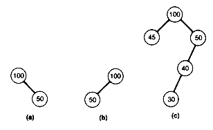
Figure 9.1 One Nonleftist and Two Leftist Trees
 lg (n + 1)
 nodes. Such a shortest path can always be obtained by traversing the right chain from the root.
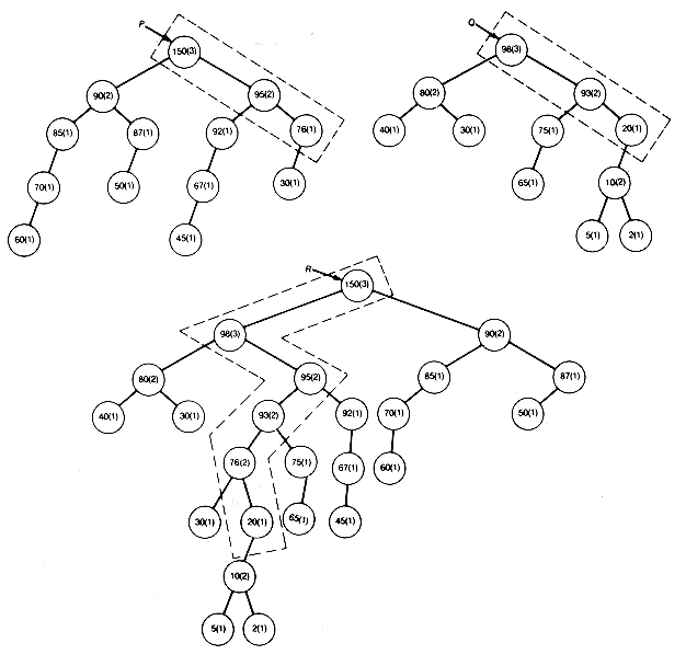
Figure 9.2 The Merging of Leftist Trees Implemented in Linked Representation
9.3: Hash Tables
9.3.1 Building a Hash Table
Table 9.2 Hash Addresses
Hashing Hashing
Key Value Address Key Value Address
---------------------------------------------
019 --> 19 468 --> 08
392 --> 01 814 --> 09
179 --> 18 720 --> 07
359 --> 14 260 --> 07
663 --> 19 802 --> 20
262 --> 09 364 --> 19
639 --> 18 976 --> 10
321 --> 22 774 --> 15
097 --> 05 566 --> 14
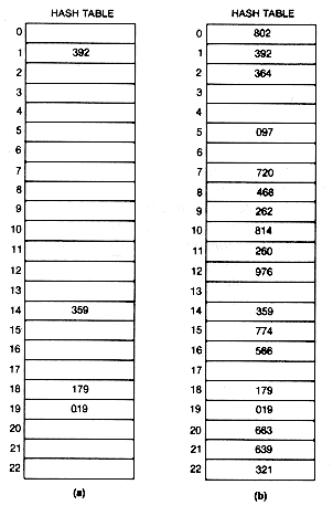
Figure 9.3 Hash Table (a) after Four Entries and (b) Finally
9.3.2 Searching a Hash Table
1/18 X 1 + 1/18 X 1 + 1/18 X 1 + 1/18 X 1 + 1/18 X 2 + 1/18 X 1
+ 1/18 X 4 + 1/18 X 1 + 1/18 X 1 + 1/18 X 1 + 1/18 X 2 + 1/18 X 1
+ 1/18 X 5 + 1/18 X 4 + 1/18 X 7 + 1/18 X 3 + 1/18 X 1 + 1/18 X 3
9.3.3 Random Hashing
 )1n 1/(1-
 ) and 1/(1-
 ) where
  = n/m. The remarkable fact is that the average search time does not depend on n, the number of records stored in the table, but only on the usage ratio, n/m. Thus storage can be traded for speed in hash table searches. For example, if n is 10,000 and m is 11,112,
  is about 0.90, and an average of only 2.56 probes will be required for a successful search. Contrast this with the 5,000 comparisons or probes needed for the linear search in the random case, or the 12.29 comparisons or probes needed for a binary search. Actual hashing functions and collision resolution policies can come close to achieving this kind of average behavior. The worst-case times for hash table searching can, however, be quite large.
Table 9.3 Average Number of Probes for Searches
Successful Unsuccessful
Usage Ratio n/m Search Search
-----------------------------------------
.25 1.15 1.33
.50 1.39 2.00
.75 1.85 4.00
.80 2.01 5.00
.90 2.56 10.00
.95 3.15 20.00
9.3.4 Other Collision Resolution Policies: Open Addressing and Chaining
 for some integer
  that is not a factor of m will give such a probe sequence. To see this, take m = 13 and
  = 5. The probe sequence is then generated by [h(k) + i X 5] mod 13 for i = 0, 1, 2, . . . , 12. If h(k) = 7, this gives the probe sequence
 = 1 and
  = 4, respectively. In addition, the number of probes required for the insertion of each key is indicated for each table. You should create these tables yourself to confirm their correctness and to aid in understanding the discussion.
 Hash Hash Hash Hash Hash Hash
Keys Address Table (a) Table (b) Table (c) Table (d) Table (e)
-----------------------------------------------------------------------
019 19 0 802 (4) 663 (2) 364 (5) 364 (4) 392 (1)
392 01 1 392 (1) 392 (1) 392 (1) 392 (1)
179 18 2 364 (7)
359 14 3 321 (2)
663 19 4 364 (3) 566 (3)
262 09 5 097 (1) 097 (1) 097 (1) 097 (1) 097 (1)
639 18 6 720 (3) 260 (3) 663 (3)
321 22 7 720 (1) 720 (1) 639 (2) 720 (1) 720 (1)
097 05 8 468 (1) 468 (1) 468 (1) 468 (1) 468 (1)
468 08 9 262 (1) 262 (1) 262 (1) 262 (1) 262 (1)
814 09 10 814 (2) 976 (1) 976 (1) 814 (2) 976 (1)
720 07 11 260 (5) 260 (2) 976 (2) 364 (2)
260 07 12 976 (3) 566 (12) 814 (3) 321 (2)
802 20 13 814 (2) 566 (3)
364 19 14 359 (1) 359 (1) 359 (1) 359 (1) 359 (1)
976 10 15 774 (1) 774 (1) 774 (1) 774 (1) 774 (1)
774 15 16 566 (3) 566 (3)
566 14 17 260 (4) 639 (3) 260 (4)
18 179 (1) 179 (1) 179 (1) 179 (1) 179 (1)
19 019 (1) 019 (1) 019 (1) 019 (1) 019 (1)
20 663 (2) 802 (1) 663 (2) 663 (2) 806 (1)
21 639 (4) 802 (2) 802 (2) 814 (2)
22 321 (1) 639 (2) 321 (1) 321 (1) 639 (2)
linear displaced secondary quadratic double
probing linear clustering residue hashing
probing
Average number 2.22 2.00 1.89 1.72 1.61
of probes for a
succesful search
Figure 9.4 Typical Hash Tables for the Five Open-Addressing Techniques Considered (Usage Ratio 78 Percent)


Linear probing 7, 8, 9, 10, 11, 12 (7)
Displaced linear
probing 7, 11, 15, 19, 0, 4, 8, 12, 16 (9)
Secondary
clustering 7, 18, 6, 17, 5, 16 (6)
Quadratic
residue 7, 8, 6, 11, 3 (5)
Double hashing 7, 9, 11, 13 (4)
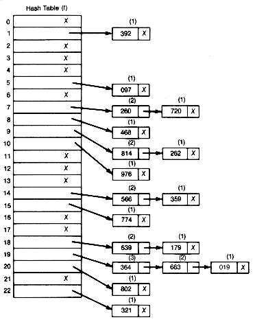
Figure 9.5 Hash Table for Separate Chaining
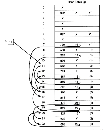
Figure 9.6 Hash Table for Coalesced Chaining
9.3.5 Searching in Ordered Hash Tables
9.3.6 Deletion from Hash Tables
9.3.7 Hashing Overview
9.4: Binary Search Trees
9.4.1 Searching the Search Trees
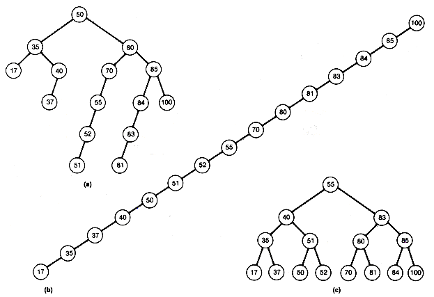
Figure 9.7 Three Binary Search Trees Containing the Same Data
typedef struct treenode
{whatever info;
struct treenode *leftptr;
struct treenode *rightptr;
}binarytreenode, *binarytreepointer;
found = FALSE;
p = t;
pred = NULL;
while ((p != NULL) && (!found))
if (keyvalue == p->key)
found = TRUE;
else if (keyvalue < p->key)
{pred = p;
p = p->leftptr;
}
else
{pred = p;
p = p->rightptr:
}
9.4.2 Growing the Search Tree "Simply"

Figure 9.8 Binary Search Tree Created from Figure 9.7
p = malloc(sizeof(binarytreenode));
p->key = keyvalue;
p->leftptr = NULL;
p->rightptr = NULL;
if (keyvalue < pred->key)
pred->leftptr = p;
else
pred->rightptr = p;
9.4.3 The Shape of Simple Binary Search Trees
 lg(n + 1)
 . Suppose the input is selected so that each of the n! possible orderings is equally likely to occur. This would be the case if the first input record is selected at random from among the n records, the second is selected at random from among the remaining n - 1 records, and so on. What will be the average depth of trees grown by the algorithm in this case? To calculate the average depth directly would mean to generate, for each of the n! orderings of input records, the binary search tree grown and note its depth. Then add up the n! depths and divide by n! to obtain the average depth.
9.4.4 Deleting a Record "Simply"
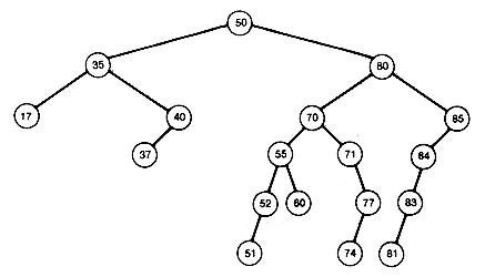
(a) Before Deletion of Records
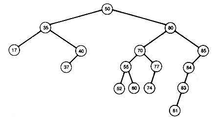
(b) After Deletion of 51 and 71
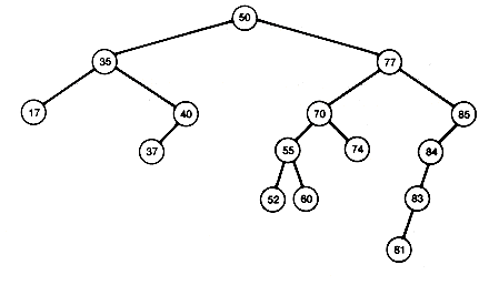
(c) After Deletion of 80
Figure 9.9 A Binary Search Tree before and after Deletion of Records
9.4.5 A Balancing Act
 , where
  . It follows from this that
  . Also, from Chapter 7, n
  2d - 1. After some manipulations we may conclude that
 lg (n + 1)
 , the worst depth of an AVL tree storing n records is at most 44 percent more than the best achievable. Contrast this with the "simple" binary search tree for which the average depth is at least 39 percent more than the best achievable; it is clearly very desirable to be able to create and use AVL trees.
9.4.6 Maintaining Balance
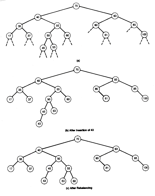
Figure 9.10 An AVL Tree before and after Insertion
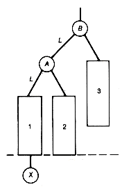
(a) Imbalance LL
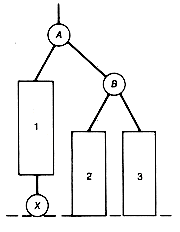
(b) Remedy for LL
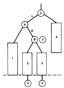
(c) Imbalance LR
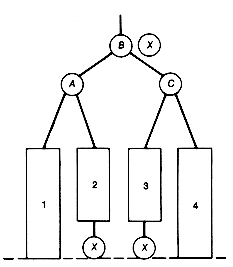
(d) Remedy for LR
Figure 9.11 Two Imbalances and Their Remedies
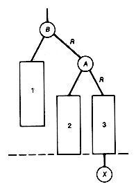
(a) Imbalance RR
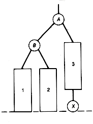
(b) Remedy for RR
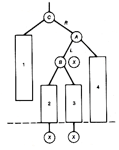
(c) Imbalance RL
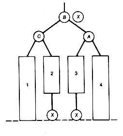
(d) Remedy for RL
Figure 9.12 Two More Imbalances and Their Remedies

Figure 9.13 Rectangles 1-3 of Figure 9.12(a) and 9.12(b)
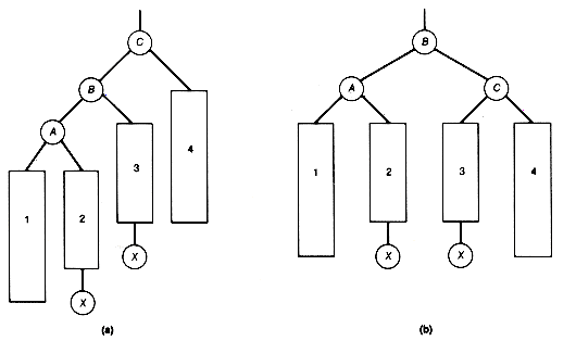
Figure 9.14 The Double Rotation Producing Remedy LR
LL: rotateright(plast) where last points to B
RR: rotateleft(plast) where last points to B
LR: rotateleft(p(last.leftptr)) where last points to C
rotateright(plast)
RL: rotateright(p(last.rightptr)) where last points to C
rotateleft(plast)
rotateright(plocalroot)
/* Performs a rotation to the right
of the subtree whose root is
pointed to by localroot.
*/
binarytreepointer *plocalroot;
{binarytreepointer q;
q = (*plocalroot).leftptr;
(*plocalroot).leftptr = q->rightptr;
q->rightptr = *plocalroot;
*plocalroot = q;
}
typedef struct treenode
{whatever key;
struct treenode *leftptr;
struct treenode *rightptr;
int balance;
}binarytreenode,*binarytreepointer;
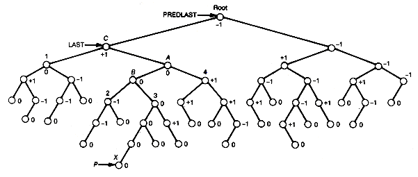
(a) Unbalanced
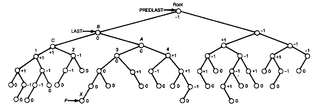
(b) Balanced
Figure 9.15 Rebalancing a Binary Tree
#define TRUE 1
#define FALSE 0
#define NULL 0
insertavl(keyvalue,pt)
/* Inserts a new record with key equal to
keyvalue in the AVL tree t, if a record
with this keyvalue is not present in t.
After insertion t will still be an AVL tree.
*/
whatever keyvalue;
binarytreepointer *pt;
{binarytreepointer p,predp,last,predlast,q;
int found;
search(keyvalue,*pt,&p,&predp,
&last,&predlast,&found);
if(!found)
{createnode(keyvalue,&p);
insertnode(keyvalue,p,predp,pt);
if(p != *pt)
if(predp->balance == 0)
if(keyvalue < last->key)
if(last->balance == 0)
{last->balance = -1;
resetpathbalances(keyvalue,
last->leftptr,p);
}
else if(last->balance == +1)
{last->balance = 0;
resetpathbalances(keyvalue,
last->leftptr,p);
}
else
{q = last->leftptr;
if(keyvalue < q->key)
ll(keyvalue,&last,p);
else
lr(keyvalue,&last,&q,p);
last->balance = 0;
if(predlast == NULL)
*pt = last;
else if(keyvalue < predlast->key)
predlast->leftptr = last;
else
predlast->rightptr = last;
}
else
if(last->balance == 0)
{last->balance = +1;
resetpathbalances(keyvalue,
last->rightptr,p);
}
else if(last->balance == -1)
{last->balance = 0;
resetpathbalances(keyvalue,
last->rightptr,p);
}
else
{q = last->rightptr;
if(keyvalue < q->key)
rr(keyvalue,&last,p);
else
rl(keyvalue,&last,&q,p);
last->balance = 0;
if(predlast == NULL)
*pt = last;
else if(keyvalue < predlast->key)
predlast->leftptr = last;
else
predlast->rightptr = last;
}
else
predp->balance = 0;
}
}
ll(keyvalue,plast,p)
/* Applies remedy ll, resets the balance of the node
involved in the remedy but not on the new search
path, and resets the proper new search path balances.
*/
whatever keyvalue;
binarytreepointer *plast,p;
{rotateright(plast);
((*plast)->rightptr)->balance = 0;
resetpathbalances(keyvalue,(*plast)->leftptr,p);
}
lr(keyvalue,plast,pq,p)
/* Applies remedy lr, resets the balance of the node
involved in the remedy but not on the new search
path, and resets the proper new search path balances.
*/
whatever keyvalue;
binarytreepointer *plast,*pq,p;
{rotateleft(&((*plast)->leftptr));
rotateright(plast);
if(keyvalue < (*plast)->key)
{(*pq).balance = 0;
((*plast)->rightptr)->balance = +1;
resetpathbalances(keyvalue,
((*plast)->leftptr)->rightptr,p);
}
else if(keyvalue > (*plast)->key)
{(*pq)->balance = -1;
((*plast)->rightptr)->balance = 0;
resetpathbalances(keyvalue,
((*plast)->rightptr)->leftptr,p);
}
else
((*plast)->rightptr)->balance = 0;
}
rr(keyvalue,plast,p)
/* Applies remedy rr, resets the balance
of the node involved in the remedy but
not on the new search path, and resets
the proper new search path balances.
*/
whatever keyvalue;
binarytreepointer *plast,p;
{rotateleft(plast);
((*plast)->leftptr)->balance = 0;
resetpathbalances(keyvalue,(*plast)->rightptr,p);
}
rl(keyvalue,plast,pq,p)
/* Applies remedy rl, resets the balance
of the node involved in the remedy but
not on the new search path, and resets
the proper new search path balances.
*/
whatever keyvalue;
binarytreepointer *plast,*pq,p;
{rotateright(&((*plast)->rightptr));
rotateleft(plast);
if(keyvalue > (*plast)->key)
{(*pq)->balance = 0;
((*plast)->leftptr)->balance = -1;
resetpathbalances(keyvalue,((*plast)->rightptr)->leftptr,p);
}
else if(keyvalue < (*plast)->key)
{(*pq)->balance = +1;
((*plast)->leftptr)->balance = 0;
resetpathbalances(keyvalue,((*plast)->leftptr)->rightptr,p);
}
else
((*plast)->leftptr)->balance = 0;
}
rotateright(plocalroot)
/* Performs a rotation to the right
of the subtree whose root is
pointed to by localroot.
*/
binarytreepointer *plocalroot;
{binarytreepointer q;
q = (*plocalroot)->leftptr;
(*plocalroot)->leftptr = q->rightptr;
q->rightptr = *plocalroot;
*plocalroot = q;
}
rotateleft(plocalroot)
/* Performs a rotation to the left
of the subtree whose root is
pointed to by localroot.
*/
binarytreepointer *plocalroot;
{binarytreepointer q;
q = (*plocalroot)->rightptr;
(*plocalroot)->rightptr = q->leftptr;
q->leftptr = *plocalroot;
*plocalroot = q;
}
resetpathbalances(keyvalue,start,p)
/* Resets the balances of all nodes on
search path between the nodes
pointed to by start and p.
*/
whatever keyvalue;
binarytreepointer start,p;
{binarytreepointer q;
q = start;
while(q !=p)
if(keyvalue < q->key)
{q-balance = -1;
q = q->leftptr;
}
else
{q->balance = +1;
q = q->rightptr;
}
}
createnode(keyvalue,pp)
/* Returns with p pointing to a new node
record with key equal to keyvalue,
left and right pointer fields null, and
balance field zero.
*/
whatever keyvalue;
binarytreepointer *pp;
{*pp = malloc(sizeof(binarytreenode));
(*pp)->key = keyvalue;
(*pp)->leftptr = NULL;
(*pp)->rightptr = NULL;
(*pp)->balance = 0;
}
search(keyvalue,t,pp,ppredp,plast,ppredlast,pfound)
/* Returns with found true only if the binary search
tree t has a node with its key equal to keyvalue.
If found is true
p and predp point respectively, to
the found node and its predecessor,
else
predp, and last, will point, respectively,
to the node that will be the new node's
predecessor, and the node along the search
path closest to the new node's insertion point
that may become unbalanced.
*/
whatever keyvalue;
binarytreepointer t,*pp,*ppredp,*plast,*ppredlast;
int *pfound;
{*pfound = FALSE;
*pp = t;
*plast = t;
*ppredp = NULL;
*ppredlast = NULL;
while((*pp != NULL) && (!*pfound))
if(keyvalue < (*pp)->key)
{if((*pp)->balance != 0)
{*ppredlast = *ppredp;
*plast = *pp;
}
*ppredp = *pp;
*pp = (*pp)->leftptr;
}
else if(keyvalue > (*pp)->key)
{if((*pp)->balance != 0)
{*ppredlast = *ppredp;
*plast = *pp;
}
*ppredp = *pp;
*pp = (*pp)->rightptr;
}
else
*pfound = TRUE;
}
insertnode(keyvalue,p,predp,pt)
/* Inserts the new node, pointed to
by p, as the proper successor
of predp.
*/
whatever keyvalue;
binarytreepointer p,predp,*pt;
{if(predp == NULL)
*pt = p;
else
if(predp == *pt)
if(keyvalue < (*pt)->key)
(*pt)->leftptr = p;
else
(*pt)->rightptr = p;
else
if(keyvalue < predp->key)
predp->leftptr = p;
else
predp->rightptr = p;
}
To insert a node in t:
If t is null then
create the new node, set its field values and set t to it
else
if keyvalue < t.key, then
insert the node in t.leftptr
if t is balanced, then
reset its balance
else
rebalance t and reset the balances of the nodes involved in the
remedy
else if keyvalue > t.key then
insert the node in t.rightptr
if t is balanced, then
reset its balance
else
rebalance t and reset the balances of the nodes involved in the
remedy.
#define TRUE 1
#define FALSE 0
#define NULL 0
insertavl(keyvalue,pt,pincrease)
/* Inserts a new record with key value to
keyvalue in the AVL tree t, if a record
with this keyvalue is not present in t.
After insertion t will still be an AVL tree.
Increase must be zero when the function is invoked.
*/
whatever keyvalue;
binarytreepointer *pt;
int *pincrease;
{binarytreepointer q;
if(*pt == NULL)
{createnode(keyvalue,pt);
*pincrease = 1;
}
else if(keyvalue < (*pt)->key)
{insertavl(keyvalue,
&((*pt)->leftptr),pincrease);
if(*pincrease) == 1)
if((*pt)->balance == 0)
(*pt)->balance = -1;
else if((*pt)->balance == +1)
{(*pt)->balance = 0;
*pincrease = 0;
}
else
{q = (*pt)->leftptr;
if(keyvalue < q->key)
ll(pt);
else
lr (pt,q);
(*pt)->balance = 0;
*pincrease = 0;
1 t's depth did not increase
}
}
else if(keyvalue > (*pt)->key)
{insertavl(keyvalue,
&((*pt)->rightptr),pincrease);
if(*pincrease == 1)
if((*pt)->balance == 0)
(*pt)->balance = +1;
else if((*pt)->balance == -1)
{(*pt)->balance = 0;
*pincrease = 0;
}
else
{q = (*pt)->rightptr;
if(keyvalue > q->key)
rr (pt)
else
rl(pt,q);
(*pt)->balance = 0;
*pincrease = 0;
}
}
}
ll(pt)
/* Apply remedy ll and reset the
balance of the node involved in
the remedy.
*/
binarytreepointer *pt;
{rotateright(pt);
reset1balance((*pt)->rightptr);
}
lr(pt,q)
/* Apply remedy lr and reset the balances
of the two nodes involved in
the remedy.
*/
binarytreepointer *pt,q;
{rotateleft(&((*pt)->leftptr));
rotateright(pt);
reset2balances(q,*pt,(*pt)->rightptr);
}
rr(pt)
/* Apply remedy rr and reset the
balance of the node involved in
the remedy.
*/
binarytreepointer *pt;
{rotateleft(pt);
reset1balance((*pt)->leftptr);
}
rl(pt,q)
/* Apply remedy rl and reset the balances
of the two nodes involved in the remedy.
*/
binarytreepointer *pt,q;
{rotateright(&((*pt)->rightptr));
rotateleft(pt);
reset2balances(q,*pt,(*pt)->leftptr);
}
rotateright(plocalroot)
/* Performs a rotation to the right
of the subtree whose root is
pointed to by localroot.
*/
binarytreepointer *plocalroot;
{binarytreepointer q;
q = (*plocalroot)->leftptr;
(*plocalroot)->leftptr = q->rightptr;
q->rightptr = *plocalroot;
*plocalroot = q;
}
rotateleft(plocalroot)
/* Performs a rotation to the left
of the subtree whose root is
pointed to by localroot.
*/
binarytreepointer *plocalroot;
{binarytreepointer q;
q = (*plocalroot)->rightptr;
(*plocalroot)->rightptr = q->leftptr;
q->leftptr = *plocalroot;
*plocalroot = q;
}
createnode(keyvalue,pp)
/* Returns with p pointing to a new node
record with key equal to keyvalue,
left and right pointer fields null, and balance field zero.
*/
whatever keyvalue;
binarytreepointer *pp;
{*pp = malloc(sizeof(binarytreenode));
(*pp)->key = keyvalue;
(*pp)->leftptr = NULL;
(*pp)->rightptr = NULL;
(*pp)->balance = 0;
}
reset1balance(q)
/* Sets the balance of node
q to zero.
*/
binarytreepointer q;
{q->balance = 0;
}
reset2balances(q,t,p)
/* Resets the balance of nodes
p and q determined by the
balance of t.
*/
binarytreepointer q,t,p;
{if(t->balance == -1)
p->balance = +1;
else
p->balance = 0;
if(t->balance == +1)
q->balance = -1;
else
q->balance = 0;
}
#include <stdio.h>
#define NULL 0
typedef int whatever;
typedef struct treenode
{whatever key;
struct treenode *leftptr;
struct treenode *rightptr;
int balance;
}binarytreenode,*binarytreepointer;
binarytreepointer left(p)
/* Returns a copy of the left pointer
of the node pointed to by p.
*/
binarytreepointer p;
{return(p->leftptr);
}
binarytreepointer right(p)
/* Returns a copy of the right pointer
of the node pointed to by p.
*/
binarytreepointer p;
{return(p->rightptr);
}
info(l)
/* Returns the key field value of
the node pointed to by l.
*/
binarytreepointer l;
{return(l->key);
}
bal(l)
/* Returns the balance field value of
the node pointed to by l.
*/
binarytreepointer l;
{return(l->balance);
}
binarytreepointer setnull()
/* Returns a null pointer. */
{return(NULL);
}
#define SENTINEL -1
main()
/* Reads record information, creates an AVL tree
storing the records, prints the key field values
of the tree records in preorder access order
after each record is inserted in the tree, and
prints the key & balance field values of the
final tree in preorder access order.
*/
{binarytreepointer t,setnull();
int keyvalue,increase;
t = setnull();
printf(\" enter keyvalue or sentinel \n");
scanf("%d",&keyvalue);while(keyvalue != SENTINEL)
}
increase = 0;
insertavl(keyvalue,&t,&increase);
printf("\n enter keyvalue or sentinel \n");scanf("%d",&keyvalue);printtree(t);
}
preorder (t);
}
printtree(t)
/* Prints the keys of t in
preorder access order.
*/
binarytreepointer t,left(),right();
{printf("\n %d \n",info(l));printtree(left(t));
printtree(right(t));
}
preorder(t)
/* Prints the keys & balances of
t in preorder access order.
*/
binarytreepointer t,left(),right(),setnull();
{if(t == setnull())
printf("\n The tree is null \n");else
{process(t);
preorder(left(t));
preorder(right(t));
}
}
process(t)
/* Prints the key and balance fields of
the node pointed to by t.
*/
binarytreepointer t;
{printf("\n key:%d balance:%d \n",info(t),bal(t));}
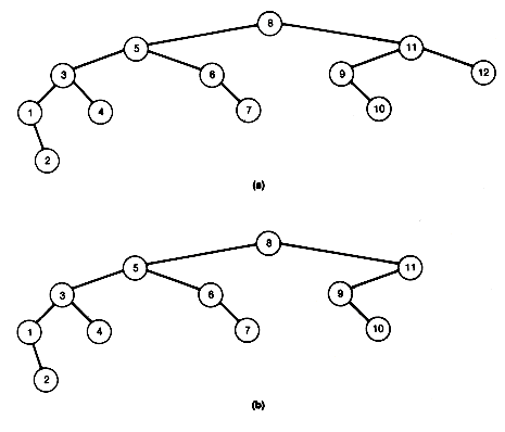
Figure 9.16 A Fibonacci Tree of Depth 5 and Deletion
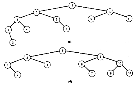
Figure 9.16
To delete a node from t:
If t is not null, then
if keyvalue<t.key, then
delete the node from t.leftptr
if t is balanced, then
reset its balance
else
rebalance t and reset balances
else if keyvalue>t.key, then
delete the node from t.rightptr
if t is balanced, then
reset its balance
else
rebalance t and reset balances
else
delete the node with the largest key value in t.leftptr
replace the root of t by that deleted node
if t is balanced, then
reset its balance
else
rebalance t and reset balances.
9.4.7 Access By Order in AVL Trees
1. 17 9. 60
2. 35 10. 70
3. 37 11. 80
4. 40 12. 81
5. 45 13. 83
6. 50 14. 85
7. 53 15. 100
8. 55
9.4.8 Binary Search Tree Overview
9.5: A Brief Review
Exercises
 key. If no such node exists, p should return with its value null.
Suggested Assignments


